import sys
import time
from functools import partial

import optax
import optuna
import numpy as np
import pandas as pd
import jax
from jax import numpy as jnp
import netket as nk
import flax
from flax import linen as nn
from netket.experimental.nn.rnn import GRU1DCell, RNNLayer
from netket.utils import struct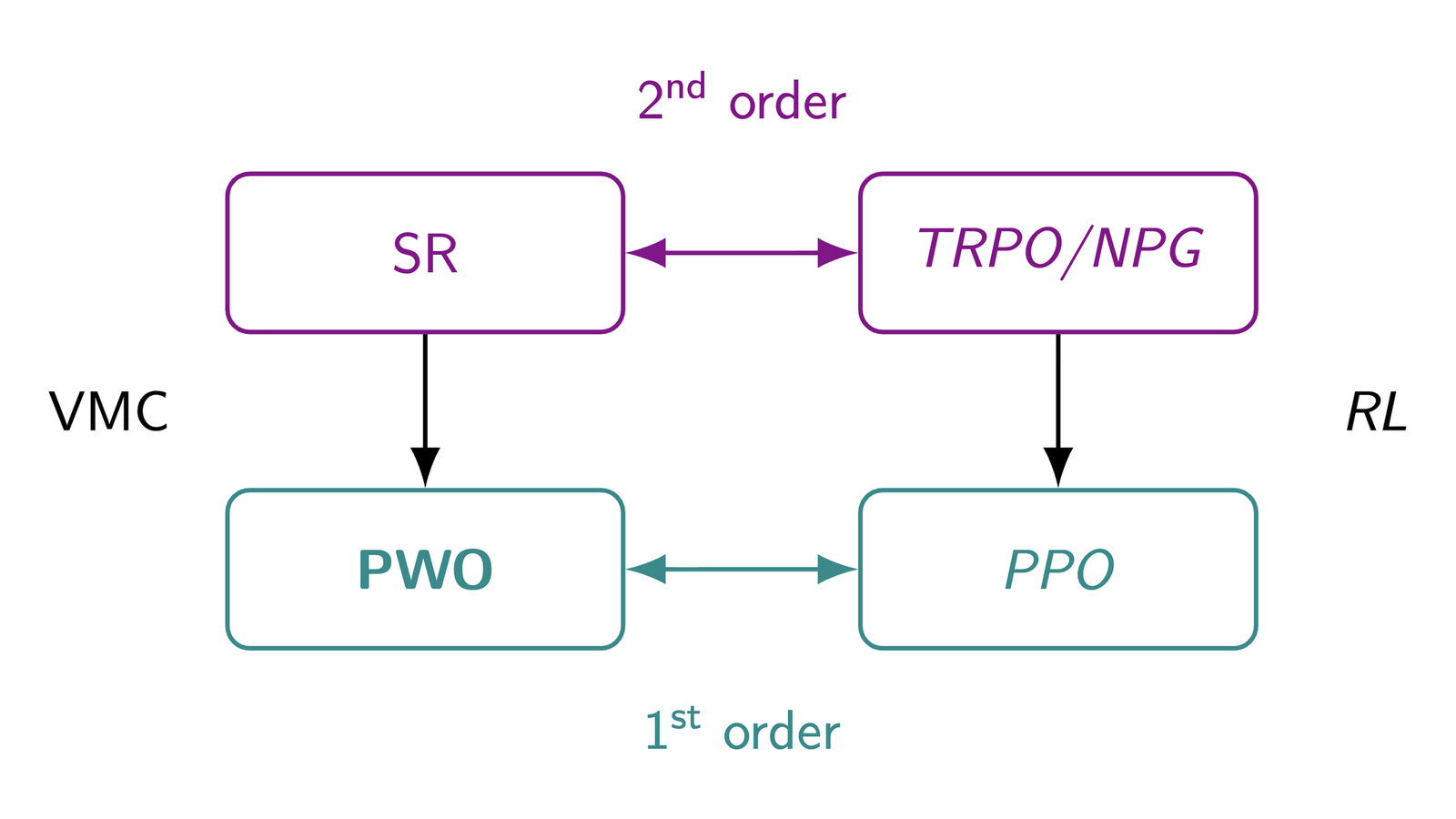
Introduction
In this post, we present Proximal Wavefunction Optimization (PWO), a novel first-order optimization algorithm for Neural Quantum States (NQS) that draws inspiration from Proximal Policy Optimization (PPO) in Reinforcement Learning (RL). PWO addresses the limitations of Stochastic Reconfiguration (SR), the standard optimizer for NQS, by enabling sample reuse and providing a more efficient optimization process.
Context
Quantum Many-Body Physics
Quantum Many-Body Physics (QMBP) studies systems of many quantum particles, where the degrees of freedom of each particle are usually simple, and the complexity arises from the interactions between them. The goal is to understand the collective behavior that emerges from these interactions, which often leads to rich phase diagrams and exotic states of matter. The study of quantum many-body systems is crucial for understanding fundamental physics and has applications in quantum computing, materials science, and condensed matter physics.
A canonical example of a quantum many-body system is the Transverse Field Ising Model (TFIM), whose Hamiltonian, i.e. the operator that defines the dynamics of the system, is the following: \[ \hat{\mathbf{H}} = -J \sum_{\langle i,j \rangle} \hat{\mathbf{S}}^{(i)}_z \hat{\mathbf{S}}^{(j)}_z - h \sum_i \hat{\mathbf{S}}^{(i)}_x, \] where \(J\) is the coupling strength between nearest-neighbor spins, \(h\) is the transverse magnetic field, \(\langle i,j \rangle\) denotes nearest-neighbor pairs and \(\hat{\mathbf{S}}^{(i)} = \pqty{\hat{\mathbf{S}}^{(i)}_x, \hat{\mathbf{S}}^{(i)}_y, \hat{\mathbf{S}}^{(i)}_z}\) are the so-called spin operators of the \(i\)-th particle. However, quantum many-body systems are not limited to spins. The common feature of all these systems is that they are described by a Hamiltonian, \(\hat{H}\), which is a Hermitian operator acting on a Hilbert space, \(\mathcal{H}\), whose dimension grows exponentially with the number of particles. We find examples of quantum many-body systems in condensed matter physics, quantum chemistry, and high-energy physics.
Ground State of a Quantum System
One of the central tasks in QMBP is to find the so-called ground state, \(\ket{\psi_0}\in\mathcal{H}\), of a given Hamiltonian, \(\hat{H}\), which can be characterized in two ways.
The first characterization is as the eigenstate, \(\ket{\psi_0}\), of \(\hat{H}\) corresponding to the lowest eigenvalue, \(E_0\), the ground-state energy. This provides a direct analytical method to find the ground state: we just need to compute the spectral decomposition of the Hamiltonian. However, this method becomes intractable very quickly due to the exponential growth of the Hilbert space \(\mathcal{H}\) where quantum states live with the number of particles. For a system of \(N\) spins (two-level particles), the Hamiltonian is a matrix with dimensions \(2^N\times 2^N\), and the complexity of performing its exact diagonalization is \(\order{2^{3N}}\).
An alternative way to define the ground state is to make use of the Variational Principle from Quantum Physics, which states that the ground state is the one that minimizes the expected value of the Hamiltonian (i.e. the energy): \[ E_0\leq E[\psi] = {\mel{\psi}{\hat{H}}{\psi}},\quad\forall\ket{\psi}\in\mathcal{H}, \] where the equality holds if and only if \(\ket{\psi}\) belongs to the ground-state eigenspace.
Variational Monte Carlo
The variational characterization of the ground state allows us to turn the problem of finding this state from a spectral decomposition problem to an optimization problem. The resulting approach receives the name of variational methods. Nevertheless, searching over the complete Hilbert space also becomes intractable quickly. For this reason, variational methods rely on two key components:
An ansatz, i.e. a parametric family of quantum states, \(\ket{\psi_{\vb*{\theta}}}\), to reduce the search space, so the problem reduces to solving \[ \vb*{\theta}^\star = \argmin_{\vb*{\theta}} E[\psi_{\vb*{\theta}}] = \argmin_{\vb*{\theta}} \frac{\langle \psi_{\vb*{\theta}} | \hat{H} | \psi_{\vb*{\theta}} \rangle}{\langle \psi_{\vb*{\theta}} | \psi_{\vb*{\theta}} \rangle}. \]
An optimizer that effectively finds the parametrization that minimizes the energy.
Despite these strategies, computing the expected value of the Hamiltonian, and potentially other related quantities like its gradient, can still be computationally expensive. A popular way to overcome this bottleneck is making use of Monte Carlo (MC) sampling to estimate these quantities. The resulting approach is called Variational Monte Carlo (VMC) (Becca and Sorella 2017).
Neural Quantum States
Regarding the ansatz in VMC, Neural Networks (NNs) (Dawid 2025) are one of the choices that is drawing more attention nowadays. The resulting method is known as Neural Quantum Wavefunctions or Neural Quantum States (NQS) (Carleo and Troyer 2017; Lange et al. 2024). The idea is to use a neural network, \(f_{\vb*{\theta}}:\{+1, -1\}^N\to\C\), to parametrize the wavefunction, \(\psi_{\vb*{\theta}}\), of the trial quantum state, \(\ket{\psi_{\vb*{\theta}}}\): \[ \ket{\psi_{\vb*{\theta}}} = \sum_{\vb{s}\in\{+1, -1\}^N}\psi_{\vb*{\theta}}(\vb{s})\ket{\vb{s}}\qq{with} \psi_{\vb*{\theta}}(\vb{s}) = f_{\vb*{\theta}}(\vb{s}). \]
The input of the model is a chain of spins \(\vb{s}\) and the output is the complex amplitude of the corresponding state in the computational basis. Note that we are restricting the discussion to spin systems, but NQS can be applied to other quantum many-body systems as well.
There are multiple reasons that support this approach: the expressivity of NNs (Hornik et al. 1989) that allows them to capture complex correlations and volume law entanglement (Deng et al. 2017), their polynomial cost with the number of particles and their effectiveness to combat the curse of dimensionality, their capacity to integrate informative priors in the form of inductive biases (like symmetries) to reduce the search space and make the solutions more physically plausible (Lange et al. 2024; Bronstein et al. 2017, 2021), their ability to be optimized using gradient-based methods (Bottou et al. 2018) via automatic differentiation (Baydin et al. 2018) and backpropagation (Rumelhart et al. 1986), and the fact that they leverage the advances of a fast-progressing field like Deep Learning (LeCun et al. 2015).
Stochastic Reconfiguration
As for the optimizer, successful NQS training often requires more sophisticated algorithms than first order methods (Bottou et al. 2018) like SGD (Robbins and Monro 1951) or Adam (Kingma and Ba 2017). These methods can suffer from slow convergence and instability due to the complex geometry of the energy landscape and the influence of MC sampling. For this reason, the standard optimizer for NQS is Stochastic Reconfiguration (SR) (Sorella 1998), the quantum version of Natural Gradient Descent (Amari 1998). This method has the advantages of a second-order optimizer, but it also presents an important bottleneck: its complexity is \(\order{P^3}\) and its memory cost, \(\order{P^2}\), where \(P\) is the number of parameters of the model. Some later refinements of this method tried to reduce this bottleneck. For example, minSR (Chen and Heyl 2024; Rende et al. 2024) reduces the complexity to \(\order{M^2P}+\order{M^3}\) and the memory cost to \(\order{MP}\), where \(M\) is the number of samples. In turn, SPRING (Goldshlager et al. 2024) applies momentum to minSR to improve its stability.
Motivation
Limitations of Neural Quantum States
NQS are a promising way to tackle the exponential complexity of quantum many-body problems. However, there are still some issues that are limiting their impact in important real-world problems. Many of these problems in NQS have to do with sampling. For example, many samples are drawn for each optimization step, but they are discarded afterwards, although they can be expensive to obtain and the quantum state may not have changed much. Moreover, optimization in the complex and noisy variational loss landscape usually requires second-order methods like minSR, but its computational cost scales with the cube of the number of samples, which makes it very expensive to perform accurate estimates of the gradient, since the main way to reduce the variance is to increase the number of samples. On the other hand, one of the two fundamental approaches to draw spin configurations is the use of Markov Chain Monte Carlo (MCMC) methods, like Metropolis-Hastings (Metropolis et al. 1953; Hastings 1970), but these methods often present difficulties to effectively explore the Hilbert space (autocorrelation, mode collapse, etc.), which makes the effective number of samples lower than expected and, therefore, these methods sample-inefficient (Wolff 1990; Del Debbio et al. 2004). Autoregressive (AR) models (Sharir et al. 2020; Hibat-Allah et al. 2020; Moss et al. 2025) are the alternative, but they have not managed to match the performance provided by state-of-the-art non-autoregressive models together with MCMC sampling, in part due to the fact that minSR is often ill-conditioned for this kind of models.
As a result of all these issues, the biggest models used for NQS, which are in the order of only 1 million parameters, can be very expensive to train and heavily rely on a careful design of their architecture and the sampling method to restrict the search of states to the sector of the Hilbert space that respects the symmetries of each specific problem (Lange et al. 2024).
Connection with Reinforcement Learning
The second pillar of the motivation of this work is the fact that, from its origins, NQS were presented as an example of Reinforcement Learning (RL). Indeed, there are some clear similarities: there are no labels to learn from, the model instead tries to optimize a certain objective via MC sampling, and these samples are drawn from the model itself, which changes as the model is updated. However, to the authors’ knowledge, this connection was never made very explicit. In general, it remains vague and, more importantly, the potential transfer of advances from RL to NQS remains underexploited.
Goal
Taking into account the limitations of NQS and the vague connection with RL, the goal of this work can be summarized as follows:
Make explicit the connection of NQS with RL and take advantage of it to bring advances from this field to overcome the limitations of SR.
In particular, the goal of this work is to design a first-order optimizer that resembles Proximal Policy Optimization (PPO) in order to:
- Combine the effectiveness of SR, a second-order method, with the efficiency of first-order methods.
- Reuse samples for multiple optimization steps.
Background
To understand the connection between NQS and RL, so that we can transfer advances from the latter to the former, we first need to introduce some background on both fields.
Variational Monte Carlo
As mentioned before, VMC (Becca and Sorella 2017) redefines the problem of finding the ground state of a quantum system from a spectral decomposition problem to an optimization problem by defining a parametric family of quantum states, \(\ket{\psi_{\vb*{\theta}}}\), using an optimizer to minimize the energy over this family, and resorting to Monte Carlo sampling to efficiently estimate the energy and its gradient. To this end, we need to rewrite the energy and its gradient as expected values over spin configurations, \(\vb{s}\), drawn from the Born distribution, \(\mathcal{P}_{\boldsymbol{\theta}}\), (using MCMC or AR models): \[ \begin{gathered} E[\psi_{\boldsymbol{\theta}}] = \frac{\langle\psi_{\boldsymbol{\theta}}|\hat{H}|\psi_{\boldsymbol{\theta}}\rangle}{\langle\psi_{\boldsymbol{\theta}}|\psi_{\boldsymbol{\theta}}\rangle} = \mathbb{E}_{\mathbf{s}\sim\mathcal{P}_{\boldsymbol{\theta}}}\!\left[E^{\mathrm{loc}}_{\boldsymbol{\theta}}(\mathbf{s})\right],\\ \nabla_{\boldsymbol{\theta}}E[\psi_{\boldsymbol{\theta}}] = \mathbb{E}_{\mathbf{s}\sim\mathcal{P}_{\boldsymbol{\theta}}}\!\left[2\,\mathrm{Re}\!\left\{\Delta E^{\mathrm{loc}}_{\boldsymbol{\theta}}(\mathbf{s})\!\left(\nabla_{\boldsymbol{\theta}}\log\psi_{\boldsymbol{\theta}}(\mathbf{s})\right)^*\right\}\right], \end{gathered} \]
where:
- \(\mathcal{P}_{\boldsymbol{\theta}}(\mathbf{s}) = |\psi_{\boldsymbol{\theta}}(\mathbf{s})|^2 / \sum_{\mathbf{s}'} |\psi_{\boldsymbol{\theta}}(\mathbf{s}')|^2\) is the Born distribution,
- \(E^{\mathrm{loc}}_{\boldsymbol{\theta}}(\mathbf{s}) = \sum_{\mathbf{s}'}\langle\mathbf{s}|\hat{H}|\mathbf{s}'\rangle\,\psi_{\boldsymbol{\theta}}(\mathbf{s}')/\psi_{\boldsymbol{\theta}}(\mathbf{s})\) is the local energy,
- \(\Delta E^{\mathrm{loc}}_{\boldsymbol{\theta}}(\mathbf{s}) = E^{\mathrm{loc}}_{\boldsymbol{\theta}}(\mathbf{s}) - \mathbb{E}_{\mathbf{s}\sim\mathcal{P}_{\boldsymbol{\theta}}}[E^{\mathrm{loc}}_{\boldsymbol{\theta}}(\mathbf{s})]\) is the centered local energy.
Keep in mind this structure of the gradient because it will appear in a similar way in RL and will be a key component to make the connection between the two fields.
On the other hand, standard first-order optimizers like SGD or Adam are often insufficient for effectively optimizing the energy, so second-order methods such as SR are commonly used. The reason is that first-order methods provide the local descent direction along which the energy decreases the most, but they do not say anything about how small the step in that direction has to be to actually minimize the energy. Moreover, a small step in parameter space can lead to a large change in Hilbert space, which in turn can substantially modify the Born distribution from which samples are drawn and destabilize the optimization process. For this reason, SR tries to find the change in the parameters, \(\delta\boldsymbol{\theta}\), that minimizes the energy, but at the same time keeps the distance with respect to the previous parameters small in terms of the infidelity, \(\mathcal{I}\), between the corresponding quantum states:
\[\delta\boldsymbol{\theta}^\star = \underset{\delta\boldsymbol{\theta}}{\arg\min}\; E[\psi_{\boldsymbol{\theta}+\delta\boldsymbol{\theta}}] - E[\psi_{\boldsymbol{\theta}}] \quad \text{s.t.} \quad \mathcal{I}(\psi_{\boldsymbol{\theta}}, \psi_{\boldsymbol{\theta}+\delta\boldsymbol{\theta}}) \leq \epsilon \in \mathbb{R}.\]
This distance between consecutive quantum states in the optimization process is approximated to second order with the Fubini-Study metric, the real part of the quantum geometric tensor, which captures the local curvature of the Hilbert space with respect to the parameters:
\[\mathbf{S} = \mathrm{Re}\!\left\{\mathrm{Cov}_{\mathbf{s}\sim\mathcal{P}_{\boldsymbol{\theta}}}\!\left[\left(\nabla_{\boldsymbol{\theta}}\log\psi_{\boldsymbol{\theta}}(\mathbf{s})\right)^*, \nabla_{\boldsymbol{\theta}}\log\psi_{\boldsymbol{\theta}}(\mathbf{s})\right]\right\}.\]
If we also approximate the energy difference to first order, then the optimal solution for the approximate problem is given by the following update rule that preconditions the gradient with the inverse of the Fubini-Study metric:
\[\boldsymbol{\theta} \leftarrow \boldsymbol{\theta} - \eta\,\mathbf{S}^{-1}\nabla_{\boldsymbol{\theta}}E[\psi_{\boldsymbol{\theta}}],\]
where \(\eta \in \mathbb{R}\) is the learning rate. At this point, the computational bottleneck of SR becomes obvious, as \(\mathbf{S}\) is a matrix of dimension \(P\times P\), with \(P\) being the number of parameters, and computing and inverting this matrix at every update can be very costly.
Reinforcement Learning
Reinforcement learning (RL) (Agarwal et al., n.d.; Graesser and Keng 2020) is a framework for sequential decision-making where an agent interacts with an environment to maximize cumulative rewards. As it happens in VMC, in RL there are not examples of optimal solutions available beforehand (there are no labels to learn), we are only able to tell whether an action taken by the agent led to a local improvement in the cumulative reward, so suboptimal strategies are not immediately penalized.
The learning loop in RL looks as follows. The agent starts at a state \(s_0\) sampled from a set \(\mathcal{S}\) according to an initial distribution \(\mu\), and at each time step \(t\):
- The agent takes an action \(a_t\) from the set of available actions \(\mathcal{A}\), sampled from a distribution \(\pi(\cdot\mid s_t)\) named the policy,
- it transitions to a new state \(s_{t+1}\in\mathcal{S}\) sampled from the transition distribution \(\mathcal{T}(\cdot\mid s_t, a_t)\),
- and receives a reward \(r_t\) sampled from the reward distribution \(\mathcal{R}(\cdot\mid s_t, a_t, s_{t+1})\).
The result after multiple interactions with the environment is a trajectory \(\tau\), i.e. the sequence of experiences \((s_t, a_t, r_t)\) of an episode. The goal is to find the policy \(\pi\) that maximizes the expected return:
\[J(\pi) = \mathbb{E}_{\tau\sim\mathcal{P}}[R_0(\tau)] \quad \text{with} \quad R_t(\tau) = \sum_{k\geq 0}\gamma^k r_{t+k},\] where \(\gamma \in [0,1]\) is the discount factor and
\[\mathcal{P}(\tau) = \mu(s_0)\prod_{t\geq 0}\pi(a_t\mid s_t)\,\mathcal{T}(s_{t+1}\mid s_t, a_t)\,\mathcal{R}(r_t\mid s_t, a_t, s_{t+1})\]
is the probability of observing the trajectory \(\tau\) under the initial state distribution \(\mu\), the policy \(\pi\), the transition distribution \(\mathcal{T}\), and the reward distribution \(\mathcal{R}\). In so-called model-free RL, \(\mathcal{T}\) and \(\mathcal{R}\) are unknown and agents have to learn from sampled experiences.
Actor-Critic Methods
One popular family of RL algorithms to learn this policy are so-called policy gradient methods. They define a parameterized policy, \(\pi_{\boldsymbol{\theta}}\), and optimize the parameters, \(\boldsymbol{\theta}\), directly with respect to the expected return, \(J(\boldsymbol{\theta})\), via gradient ascent. A refinement of this idea are actor-critic methods.
The fundamental idea is that the gradient of the objective can be expressed as:
\[\nabla_{\boldsymbol{\theta}}J(\boldsymbol{\theta}) \propto \E_{s\sim \mathcal{V}_{\vb*{\theta}}, a\sim\pi_{\vb*{\theta}}}\!\left[\left(Q^{\pi_{\boldsymbol{\theta}}}(s,a) - b(s)\right)\nabla_{\boldsymbol{\theta}}\log\pi_{\boldsymbol{\theta}}(a\mid s)\right]\]
with \(\mathcal{V}_{\boldsymbol{\theta}}\) the state visitation distribution under the policy \(\pi_{\boldsymbol{\theta}}\), \(Q^{\pi_{\boldsymbol{\theta}}}(s,a) = \mathbb{E}_{\tau\sim\mathcal{P}_{\boldsymbol{\theta}}\mid s_0=s,a_0=a}[R_0(\tau)]\) the so-called action-value function, i.e. the expected return starting from state \(s\) and action \(a\), and \(b\) any suitable action-independent baseline. Choosing \(b(s)\) as the so-called value function \(V^{\pi_{\boldsymbol{\theta}}}(s) = \mathbb{E}_{a\sim\pi_{\boldsymbol{\theta}}}[Q^{\pi_{\boldsymbol{\theta}}}(s,a)]\), the objective can be redefined in the following way and still yield an unbiased gradient estimate of the original objective:
\[J^{\mathrm{AC}}(\boldsymbol{\theta}) = \E_{s\sim \mathcal{V}_{\vb*{\theta}}, a\sim\pi_{\vb*{\theta}}}\!\left[A^{\pi_{\boldsymbol{\theta}}}(s,a)\log\pi_{\boldsymbol{\theta}}(a\mid s)\right]\]
where \(A^{\pi_{\boldsymbol{\theta}}}(s,a) = Q^{\pi_{\boldsymbol{\theta}}}(s,a) - V^{\pi_{\boldsymbol{\theta}}}(s)\) is the so-called advantage. The motivation behind these methods is that \(A^{\pi_{\boldsymbol{\theta}}}\), \(Q^{\pi_{\boldsymbol{\theta}}}\) and \(V^{\pi_{\boldsymbol{\theta}}}\) can be estimated with learnable functions and provide a more informative reinforcing signal than just rewards, which are generally sparse and delayed signals.
Monotonic Improvement Theory
Directly optimizing \(J^{\mathrm{AC}}\) can be problematic for two important reasons. First, it is sample-inefficient: at each optimization step, all experiences obtained with past versions of the policy must be discarded and new experiences must be collected. Second, it can suffer from performance collapse: even small changes in the parameters can lead to large updates to the policy that drastically reduce performance, from which recovery may be difficult.
The solution is provided by the monotonic improvement theory, which underlies algorithms like Conservative Policy Iteration (CPI) (Kakade and Langford 2002). The cornerstone of this theory is the following inequality that sets a lower bound on the difference in performance between two policy parameterizations:
\[J(\boldsymbol{\theta}) - J(\boldsymbol{\theta}_{\mathrm{old}}) \geq \E_{s\sim \mathcal{V}_{\vb*{\theta}_{\mathrm{old}}}, a\sim\pi_{\vb*{\theta}_{\mathrm{old}}}}\!\left[r_{\boldsymbol{\theta}}A^{\pi_{\boldsymbol{\theta}_{\mathrm{old}}}}\right] - C\sqrt{\mathbb{E}_{s\sim\mathcal{V}_{\boldsymbol{\theta}_{\mathrm{old}}}}\!\left[D_{\mathrm{KL}}\!\left(\pi_{\boldsymbol{\theta}}\|\pi_{\boldsymbol{\theta}_{\mathrm{old}}}\right)\right]},\]
with \(r_{\boldsymbol{\theta}}(a, s) = \pi_{\boldsymbol{\theta}}(a\mid s)/\pi_{\boldsymbol{\theta}_{\mathrm{old}}}(a\mid s)\) the importance sampling (IS) ratio between the new and old policies and \(C\) a positive problem-dependent constant. Therefore, if we solve \[\vb*{\theta}^\star = \argmax_{\vb*{\theta}} J^{\mathrm{CPI}}_{\vb*{\theta}_{\mathrm{old}}}(\vb*{\theta}) - C\sqrt{\E_{s\sim \mathcal{V}_{\vb*{\theta}_{\mathrm{old}}}}\bqty{D_{\mathrm{KL}}\pqty{\pi_{\vb*{\theta}}\|\pi_{\vb*{\theta}_{\mathrm{old}}}}}},\]
where
\[J^{\mathrm{CPI}}_{\vb*{\theta}_{\mathrm{old}}}(\vb*{\theta}) = \E_{s\sim \mathcal{V}_{\vb*{\theta}_{\mathrm{old}}}, a\sim\pi_{\vb*{\theta}_{\mathrm{old}}}}\!\left[r_{\vb*{\theta}}A^{\pi_{\vb*{\theta}_{\mathrm{old}}}}\right]\]
is the so-called surrogate objective, we can
- ensure monotonic improvement, i.e. \(J(\vb*{\theta}^\star) - J(\vb*{\theta}_{\mathrm{old}}) \geq 0\),
- and reuse past experiences from previous policies thanks to importance sampling.
In fact, if samples are not reused from previous policies, this approach is equivalent to policy gradient ascent:
\[\eval{\grad_{\vb*{\theta}} J^{\mathrm{CPI}}_{\vb*{\theta}_{\mathrm{old}}}(\vb*{\theta})}_{\vb*{\theta}_{\mathrm{old}}} = \eval{\grad_{\vb*{\theta}} J^{\mathrm{AC}}(\vb*{\theta})}_{\vb*{\theta}_{\mathrm{old}}}.\]
Trust Region Methods
Despite its solid motivation, solving the previous problem is hard in practice because it is difficult to balance the two terms it involves: maximizing the surrogate objective while keeping the KL divergence small. A practical way to try to solve it is to define a trust region in policy space. In other words, we restrict the policy updates to stay within a certain “distance” from the current policy, measured by the KL divergence, so that we can focus on optimizing the surrogate objective:
\[\boldsymbol{\theta}^\star = \underset{\boldsymbol{\theta}}{\arg\max}\; J^{\mathrm{CPI}}_{\boldsymbol{\theta}_{\mathrm{old}}}(\boldsymbol{\theta}) \quad \text{s.t.} \quad \mathbb{E}_{s\sim\mathcal{V}_{\boldsymbol{\theta}_{\mathrm{old}}}}\!\left[D_{\mathrm{KL}}\!\left(\pi_{\boldsymbol{\theta}}\|\pi_{\boldsymbol{\theta}_{\mathrm{old}}}\right)\right] \leq \delta \in \mathbb{R}.\]
The KL divergence can be approximated to second order with the Fisher information matrix:
\[\mathbf{F} = \E_{s\sim \mathcal{V}_{\vb*{\theta}_{\mathrm{old}}}, a\sim\pi_{\vb*{\theta}_{\mathrm{old}}}}\bqty{\eval{\grad_{\vb*{\theta}}\log\pi_{\vb*{\theta}}}_{\vb*{\theta}_{\mathrm{old}}}\eval{\grad_{\vb*{\theta}}\log\pi_{\vb*{\theta}}}_{\vb*{\theta}_{\mathrm{old}}}^\top}.\]
If we also approximate the surrogate objective to first order, then the optimal solution for the approximate problem is given by the Natural Policy Gradient (NPG) (Kakade 2001) update rule:
\[\boldsymbol{\theta} \leftarrow \boldsymbol{\theta} + \eta\,\mathbf{F}^{-1}_{\mathrm{old}}\,\nabla_{\boldsymbol{\theta}}J^{\mathrm{CPI}}_{\boldsymbol{\theta}_{\mathrm{old}}}(\boldsymbol{\theta}).\]
Trust Region Policy Optimization (TRPO) (Schulman et al. 2015) is based on the same update rule, but it enforces the original trust-region constraint (not the approximate one) explicitly via backtracking line search. Both methods present the advantages of a second order optimization method, like faster and more stable convergence, but also the disadvantages, such as higher computational cost and implementation complexity. The bottleneck here is the same that is present in SR for VMC: the need to compute and invert the Fisher information matrix, which can be computationally expensive for high-dimensional parameter spaces.
Proximal Policy Optimization
Proximal Policy Optimization (PPO) (Schulman et al. 2017) is a first-order method that tries to solve the trust-region constrained policy optimization problem with simple yet effective heuristics. This method has replaced NPG and TRPO in many practical applications due to its simplicity and efficiency. In fact, it has become one of the most popular policy optimization algorithms in modern RL.
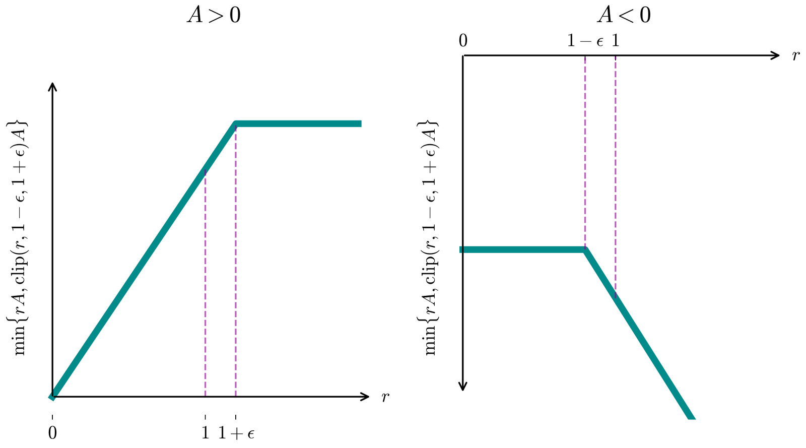
PPO redefines the objective by clipping the IS ratio in the surrogate objective and taking the minimum between the clipped and unclipped objectives:
\[J^{\mathrm{clip}}_{\boldsymbol{\theta}_{\mathrm{old}}}(\boldsymbol{\theta}) = \E_{s\sim \mathcal{V}_{\vb*{\theta}_{\mathrm{old}}}, a\sim\pi_{\vb*{\theta}_{\mathrm{old}}}}\!\left[\min\!\left(r_{\boldsymbol{\theta}}A^{\pi_{\boldsymbol{\theta}_{\mathrm{old}}}},\;r_{\boldsymbol{\theta}}^{\mathrm{clip}}\,A^{\pi_{\boldsymbol{\theta}_{\mathrm{old}}}}\right)\right],\] where \[r_{\boldsymbol{\theta}}^{\mathrm{clip}} = \operatorname{clip}(r_{\boldsymbol{\theta}}, 1-\epsilon, 1+\epsilon).\] As a result, \(J^{\mathrm{clip}}_{\vb*{\theta}_{\mathrm{old}}}\) makes the objective pessimistic about performance far away from \(\vb*{\theta}_{\mathrm{old}}\), which removes the incentive for large policy updates. Specifically, for each experience, once the importance-sampling ratio \(r_{\boldsymbol{\theta}}\) moves outside the interval \([1-\epsilon,1+\epsilon]\) in the direction that would further improve the surrogate objective, the clipping mechanism makes the corresponding gradient contribution zero. Thus, once the probability of a particular state-action pair has changed sufficiently far from the reference policy in such a direction, that experience no longer contributes to pushing its probability further away from the reference1. In this sense, the hyperparameter \(\epsilon\) controls the effective size of the trust region in practice.
Proximal Wavefunction Optimization
Advantage policy gradient framework of RL maps naturally to VMC optimization. In both cases we try to optimize a certain quantity over a parameterized model, we estimate this quantity via MC sampling, using the model itself to draw the samples, and we use gradient-based methods to update the model parameters. In Table 1, the correspondence between RL and VMC is summarized. In fact, this correspondence is exact for real and non-negative wavefunctions, like the ground states of stoquastic Hamiltonians2. In this case, we can assume \(f_{\boldsymbol{\theta}} = \log\psi_{\boldsymbol{\theta}} = \log|\psi_{\boldsymbol{\theta}}|\), and the gradient of the variational energy simplifies to3:
\[\nabla_{\boldsymbol{\theta}}E[\psi_{\boldsymbol{\theta}}] = \mathbb{E}_{\mathbf{s}\sim\mathcal{P}_{\boldsymbol{\theta}}}\!\left[\Delta E^{\mathrm{loc}}_{\boldsymbol{\theta}}(\mathbf{s})\,\nabla_{\boldsymbol{\theta}}\log\mathcal{P}_{\boldsymbol{\theta}}(\mathbf{s})\right].\]
In particular, variational energy minimization is equivalent to an advantage policy-gradient update over spin configurations in this case.
| Reinforcement Learning | Variational Monte Carlo |
|---|---|
| Action: \(a\) | Spin configuration: \(\mathbf{s}\) |
| Policy: \(\pi_{\boldsymbol{\theta}}(a\mid s)\) | Born distribution: \(\mathcal{P}_{\boldsymbol{\theta}}(\mathbf{s})\) |
| Advantage: \(A^{\pi_{\boldsymbol{\theta}}}(s,a)\) | Centered local energy: \(\Delta E^{\mathrm{loc}}_{\boldsymbol{\theta}}(\mathbf{s})\) |
| Policy gradient: \(A^{\pi_{\boldsymbol{\theta}}}\nabla_{\boldsymbol{\theta}}\log\pi_{\boldsymbol{\theta}}\) | Force: \(2\,\mathrm{Re}\!\left\{\Delta E^{\mathrm{loc}}_{\boldsymbol{\theta}}\pqty{\nabla_{\boldsymbol{\theta}}\log\psi_{\boldsymbol{\theta}}}^\ast\right\}\) |
| KL divergence: \(D_{\mathrm{KL}}(\pi_{\boldsymbol{\theta}}\|\pi_{\boldsymbol{\theta}_{\mathrm{old}}})\) | Infidelity: \(\mathcal{I}(\psi_{\boldsymbol{\theta}}, \psi_{\boldsymbol{\theta}_{\mathrm{old}}})\) |
| Fisher matrix: \(\mathbf{F}\) | Fubini-Study metric: \(\mathbf{S}\) |
Moreover, NPG and TRPO are in perfect analogy with SR, replacing the wavefunction with the policy and the Fubini-Study metric with the Fisher information matrix. This motivates the extension to NQS of PPO, which allows for sample reuse and overcomes the limitations of NPG and TRPO with a first-order approach that preserves their trust-region philosophy via simple yet effective heuristics. The aim is to overcome the problems of SR as PPO successfully did with NPG and TRPO.
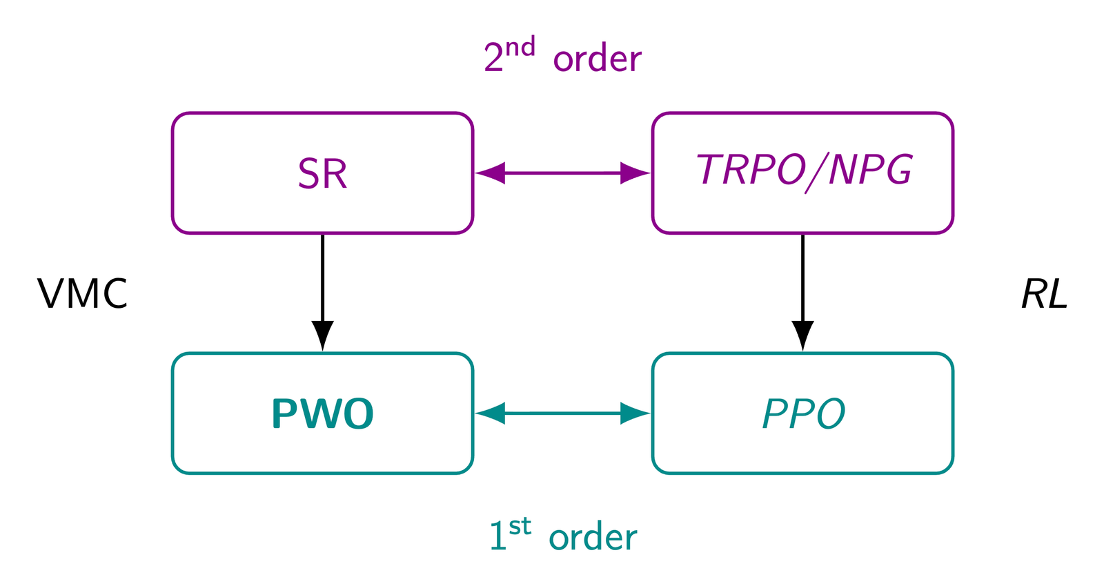
The proposed method, Proximal Wavefunction Optimization (PWO), does exactly this. The starting point is showing that the VMC gradient can be split into real and imaginary components as \[ \grad_{\vb*{\theta}} E[\psi_{\vb*{\theta}}] = \E_{\vb{s}\sim\mathcal{P}_{\vb*{\theta}}}\bqty{2A_{\vb*{\theta}}^{\mathrm{R}}(\vb{s})\grad_{\vb*{\theta}}\log\abs{\psi_{\vb*{\theta}}}} + \E_{\vb{s}\sim\mathcal{P}_{\vb*{\theta}}}\bqty{2A_{\vb*{\theta}}^{\mathrm{I}}(\vb{s})\grad_{\vb*{\theta}}\arg{\psi_{\vb*{\theta}}}}, \tag{1}\] where \(A_{\vb*{\theta}}^{\mathrm{R}}(\vb{s}) \equiv \Re\Bqty{\Delta E^{\mathrm{loc}}_{\vb*{\theta}}(\mathbf{s})}\) and \(A_{\vb*{\theta}}^{\mathrm{I}}(\vb{s}) \equiv \Im\Bqty{\Delta E^{\mathrm{loc}}_{\vb*{\theta}}(\mathbf{s})}\).
Proof. Substituting \[ \Delta E^{\mathrm{loc}}_{\boldsymbol{\theta}}(\vb{s}) = A_{\vb*{\theta}}^{\mathrm{R}}(\vb{s})+iA_{\vb*{\theta}}^{\mathrm{I}}(\vb{s}) \] and \[ \log\psi_{\boldsymbol{\theta}}(\vb{s}) = \log\abs{\psi_{\boldsymbol{\theta}}(\vb{s})} +i\arg\psi_{\boldsymbol{\theta}}(\vb{s}) \] into the VMC gradient and taking the real part gives immediately the desired decomposition.
Then, we realize that each component has the same structure and is analogous to the advantage policy gradient from RL. For this reason, a clipped surrogate objective for each component analogous to the one that PPO introduces for the policy gradient is proposed: \[ L_{\mathrm{PWO}}(\vb*{\theta}; \vb*{\theta}_{\mathrm{old}}) = L^{\mathrm{clip}}_{\mathrm{mod}}(\vb*{\theta}; \vb*{\theta}_{\mathrm{old}}) + L_{\mathrm{arg}}^{\mathrm{clip}}(\vb*{\theta}; \vb*{\theta}_{\mathrm{old}}). \] For the modulus component, \[ L^{\mathrm{clip}}_{\mathrm{mod}}(\vb*{\theta}; \vb*{\theta}_{\mathrm{old}}) = \E_{\vb{s} \sim \mathcal{P}_{{\vb*{\theta}}_{\mathrm{old}}}} \left[ \max\left(r_{\vb*{\theta}}(\vb{s}) A_{\vb*{\theta}_{\mathrm{old}}}^{\mathrm{R}}(\mathbf{s}), r^{\mathrm{clip}}_{\vb*{\theta}}(\vb{s})A_{\vb*{\theta}_{\mathrm{old}}}^{\mathrm{R}}(\mathbf{s}) \right) \right], \] where \[ r_{\vb*{\theta}}(\vb{s}) = {\mathcal{P}_{{\vb*{\theta}}}(\vb{s})}/{\mathcal{P}_{{\vb*{\theta}}_{\mathrm{old}}}(\vb{s})} \] is the importance sampling ratio between the current and reference distributions4 and \[ r^{\mathrm{clip}}_{\vb*{\theta}}(\vb{s}) = \operatorname{clip}\big(r_{\vb*{\theta}}(\vb{s}), 1-\epsilon_{\mathrm{mod}}, 1+\epsilon_{\mathrm{mod}}\big) \] is its clipped version, with \(\epsilon_{\mathrm{mod}}\in[0,1]\) the modulus-clipping threshold. For the phase component, \[ L_{\mathrm{arg}}^{\mathrm{clip}}(\vb*{\theta}; \vb*{\theta}_{\mathrm{old}}) = \E_{\vb{s}\sim \mathcal{P}_{\vb*{\theta}_{\mathrm{old}}}} \left[ \operatorname{sg}\pqty{r_{\vb*{\theta}}(\vb{s})} \max\left( \phi_{\vb*{\theta}}(\vb{s})A_{\vb*{\theta}_{\mathrm{old}}}^{\mathrm{I}}(\vb{s}), \phi^{\mathrm{clip}}_{\vb*{\theta}}(\vb{s})A_{\vb*{\theta}_{\mathrm{old}}}^{\mathrm{I}}(\vb{s}) \right) \right], \] where \(\operatorname{sg}(\cdot)\) denotes the stop-gradient operator, which detaches its input from the gradient computation; \[ \phi_{\vb*{\theta}}(\vb{s}) = 2\atan_2\pqty{\sin\pqty{\arg\psi_{\vb*{\theta}}-\arg\psi_{\vb*{\theta}_{\mathrm{old}}}}, \cos\pqty{\arg\psi_{\vb*{\theta}}-\arg\psi_{\vb*{\theta}_{\mathrm{old}}}}} \] is twice the phase difference wrapped modulo \(2\pi\) and \[ \phi^{\mathrm{clip}}_{\vb*{\theta}}(\vb{s}) = \operatorname{clip}\big(\phi_{\vb*{\theta}}(\vb{s}),-\epsilon_{\mathrm{arg}},\epsilon_{\mathrm{arg}}\big) \] is its clipped version, with \(\epsilon_{\mathrm{arg}}\in\bqty{0, \pi}\) the phase-clipping threshold. The clipping mechanism removes the incentive to move the modulus or phase of each sample farther from its reference once the corresponding modulus or phase change, respectively, exceeds its clipping threshold in the direction that would further decrease the surrogate objective.
The gradient of this objective is consistent with the original one every time we sample new spin configurations from the current parametrization of the wavefunction: \[ \eval{\grad_{\vb*{\theta}}L_{\mathrm{PWO}}(\vb*{\theta}; \vb*{\theta}_{\mathrm{old}})}_{\vb*{\theta}=\vb*{\theta}_{\mathrm{old}}} = \eval{\grad_{\vb*{\theta}}E[\psi_{\vb*{\theta}}]}_{\vb*{\theta}=\vb*{\theta}_{\mathrm{old}}}. \]
Proof. At \(\vb*{\theta}=\vb*{\theta}_{\mathrm{old}}\), we have \[ \eval{\grad_{\vb*{\theta}} L^{\mathrm{clip}}_{\mathrm{mod}}(\vb*{\theta}; \vb*{\theta}_{\mathrm{old}})}_{\vb*{\theta}=\vb*{\theta}_{\mathrm{old}}} = \eval{\grad_{\vb*{\theta}}S_{\mathrm{mod}}(\vb*{\theta};\vb*{\theta}_{\mathrm{old}})}_{\vb*{\theta}=\vb*{\theta}_{\mathrm{old}}}, \] and \[ \eval{\grad_{\vb*{\theta}} L^{\mathrm{clip}}_{\mathrm{arg}}(\vb*{\theta}; \vb*{\theta}_{\mathrm{old}})}_{\vb*{\theta}=\vb*{\theta}_{\mathrm{old}}} =\eval{\grad_{\vb*{\theta}}S_{\mathrm{arg}}(\vb*{\theta};\vb*{\theta}_{\mathrm{old}})}_{\vb*{\theta}=\vb*{\theta}_{\mathrm{old}}}, \] so, according to Theorem 3 in Section 6.1 (see the appendix), \[ \eval{\grad_{\vb*{\theta}}L_{\mathrm{PWO}}(\vb*{\theta}; \vb*{\theta}_{\mathrm{old}})}_{\vb*{\theta}=\vb*{\theta}_{\mathrm{old}}} = \eval{\grad_{\vb*{\theta}}E[\psi_{\vb*{\theta}}]}_{\vb*{\theta}=\vb*{\theta}_{\mathrm{old}}}. \]
Moreover, similar to the monotonic improvement guarantees offered by trust-region methods like CPI, NPG, TRPO or PPO from RL, PWO is supported by the following upper bound on the energy difference between two parametrizations of the wavefunction: \[ E[\psi_{\vb*{\theta}}]-E[\psi_{\vb*{\theta}_{\mathrm{old}}}]\leq L_{\mathrm{PWO}}(\vb*{\theta}; \vb*{\theta}_{\mathrm{old}}) + C_{\vb*{\theta}_{\mathrm{old}}}\mathcal{I}(\psi_{\vb*{\theta}}, \psi_{\vb*{\theta}_{\mathrm{old}}}), \]
with \[ C_{\vb*{\theta}_{\mathrm{old}}} = 2\pqty{\norm{\hat H-E[\psi_{\vb*{\theta}_{\mathrm{old}}}]\I}_{\infty} + \norm{A_{\vb*{\theta}_{\mathrm{old}}}^{\mathrm{R}}}_{\infty} + 4\pi^2\norm{A_{\vb*{\theta}_{\mathrm{old}}}^{\mathrm{I}}}_{\infty}}. \]
Proof. The energy upper bound follows from Equation 14 in Theorem 2 (see Section 6.1 in the appendix) and the pointwise inequalities \[ L^{\mathrm{clip}}_{\mathrm{mod}}(\vb*{\theta}; \vb*{\theta}_{\mathrm{old}}) \geq S_{\mathrm{mod}}(\vb*{\theta};\vb*{\theta}_{\mathrm{old}}) \qq{and} L^{\mathrm{clip}}_{\mathrm{arg}}(\vb*{\theta}; \vb*{\theta}_{\mathrm{old}}) \geq S_{\mathrm{arg}}(\vb*{\theta};\vb*{\theta}_{\mathrm{old}}), \] which hold because each clipped objective takes the maximum of the unclipped term and its clipped counterpart, and \(\operatorname{sg}(r)\) has the same forward value as \(r\).
This means that, as long as the infidelity between consecutive updates of the wavefunction in the optimization process is kept small enough, minimizing the PWO objective yields a monotonic decrease in energy. Moreover, if \(r_{\vb*{\theta}}(\vb{s})\in [1-\epsilon_{\mathrm{mod}}, 1+\epsilon_{\mathrm{mod}}]\) and \(\phi_{\vb*{\theta}}(\vb{s})\in [-\epsilon_{\mathrm{arg}},\epsilon_{\mathrm{arg}}]\) for all \(\vb{s}\), which PWO encourages but does not guarantee5, then infidelity presents the following upper bound: \[ \mathcal{I}(\psi_{\vb*{\theta}}, \psi_{\vb*{\theta}_{\mathrm{old}}})\leq\pqty{1-\frac{1+\sqrt{1-\epsilon_{\mathrm{mod}}^2}}{2}\cos^2\frac{\epsilon_{\mathrm{arg}}}{2}}, \] which behaves as \((\epsilon_{\mathrm{mod}}^2 + \epsilon_{\mathrm{arg}}^2)/4 + \order{\epsilon_{\mathrm{mod}}^4+\epsilon_{\mathrm{mod}}^2\epsilon_{\mathrm{arg}}^2+\epsilon_{\mathrm{arg}}^4}\) for small \(\epsilon_{\mathrm{mod}}\) and \(\epsilon_{\mathrm{arg}}\).
Proof. For simplicity, consider that \(\ket{\psi_{\boldsymbol{\theta}_{\mathrm{old}}}}\) and \(\ket{\psi_{\boldsymbol{\theta}}}\) are both normalized. Then, infidelity is given by
\[ \mathcal{I}\pqty{\psi_{\boldsymbol{\theta}},\psi_{\boldsymbol{\theta}_{\mathrm{old}}}} = 1- \abs{ \braket{\psi_{\boldsymbol{\theta}_{\mathrm{old}}}}{\psi_{\boldsymbol{\theta}}} }^2 \]
and the overlap can be expressed as an expectation over the reference Born distribution:
\[ \braket{\psi_{\boldsymbol{\theta}_{\mathrm{old}}}}{\psi_{\boldsymbol{\theta}}} = \sum_{\mathbf{s}} \abs{\psi_{\boldsymbol{\theta}_{\mathrm{old}}}(\mathbf{s})}^2 \frac{\psi_{\boldsymbol{\theta}}(\mathbf{s})} {\psi_{\boldsymbol{\theta}_{\mathrm{old}}}(\mathbf{s})} = \mathbb{E}_{\mathbf{s}\sim\mathcal{P}_{\boldsymbol{\theta}_{\mathrm{old}}}} \left[ \sqrt{r_{\boldsymbol{\theta}}(\mathbf{s})} \exp\!\left( \frac{i}{2}\phi_{\boldsymbol{\theta}}(\mathbf{s}) \right) \right]. \]
Taking the real part gives
\[ \mathrm{Re}\!\left[ \braket{\psi_{\boldsymbol{\theta}_{\mathrm{old}}}}{\psi_{\boldsymbol{\theta}}} \right] = \mathbb{E}_{\mathbf{s}\sim\mathcal{P}_{\boldsymbol{\theta}_{\mathrm{old}}}} \left[ \sqrt{r_{\boldsymbol{\theta}}(\mathbf{s})} \cos\!\left( \frac{\phi_{\boldsymbol{\theta}}(\mathbf{s})}{2} \right) \right]. \]
Under the assumptions that \(\abs{\phi_{\boldsymbol{\theta}}(\mathbf{s})}\leq\epsilon_{\mathrm{arg}}\) and \(\epsilon_{\mathrm{arg}}\in[0,\pi]\), we have
\[ \cos\!\left( \frac{\phi_{\boldsymbol{\theta}}(\mathbf{s})}{2} \right) \geq \cos\!\left(\frac{\epsilon_{\mathrm{arg}}}{2}\right), \]
and therefore
\[ \abs{ \braket{\psi_{\boldsymbol{\theta}_{\mathrm{old}}}}{\psi_{\boldsymbol{\theta}}} } \geq \mathrm{Re}\!\left[ \braket{\psi_{\boldsymbol{\theta}_{\mathrm{old}}}}{\psi_{\boldsymbol{\theta}}} \right] \geq \cos\!\left(\frac{\epsilon_{\mathrm{arg}}}{2}\right) \mathbb{E}_{\mathbf{s}\sim\mathcal{P}_{\boldsymbol{\theta}_{\mathrm{old}}}} \left[ \sqrt{r_{\boldsymbol{\theta}}(\mathbf{s})} \right]. \]
It remains to lower-bound the expectation of \(\sqrt{r_{\boldsymbol{\theta}}}\). Since \(r_{\boldsymbol{\theta}}(\mathbf{s})\in[1-\epsilon_{\mathrm{mod}},1+\epsilon_{\mathrm{mod}}]\), with \(0\leq\epsilon_{\mathrm{mod}}\leq1\), and
\[ \mathbb{E}_{\mathbf{s}\sim\mathcal{P}_{\boldsymbol{\theta}_{\mathrm{old}}}} \left[ r_{\boldsymbol{\theta}}(\mathbf{s}) \right] = \sum_{\mathbf{s}} \mathcal{P}_{\boldsymbol{\theta}_{\mathrm{old}}}(\mathbf{s}) \frac{\mathcal{P}_{\boldsymbol{\theta}}(\mathbf{s})} {\mathcal{P}_{\boldsymbol{\theta}_{\mathrm{old}}}(\mathbf{s})} = 1, \]
the concavity of the square-root function implies that, on the interval \([1-\epsilon_{\mathrm{mod}},1+\epsilon_{\mathrm{mod}}]\), \(\sqrt{r}\) lies above the chord joining the two endpoints. Hence
\[ \sqrt{r} \geq \frac{1+\epsilon_{\mathrm{mod}}-r}{2\epsilon_{\mathrm{mod}}}\sqrt{1-\epsilon_{\mathrm{mod}}} + \frac{r-(1-\epsilon_{\mathrm{mod}})}{2\epsilon_{\mathrm{mod}}}\sqrt{1+\epsilon_{\mathrm{mod}}}. \]
Taking the expectation and using \(\mathbb{E}[r]=1\) yields
\[ \mathbb{E}_{\mathbf{s}\sim\mathcal{P}_{\boldsymbol{\theta}_{\mathrm{old}}}} \left[ \sqrt{r_{\boldsymbol{\theta}}(\mathbf{s})} \right] \geq \frac{\sqrt{1-\epsilon_{\mathrm{mod}}}+\sqrt{1+\epsilon_{\mathrm{mod}}}}{2}. \]
Therefore,
\[ \abs{ \braket{\psi_{\boldsymbol{\theta}_{\mathrm{old}}}}{\psi_{\boldsymbol{\theta}}} }^2 \geq \frac{ \pqty{\sqrt{1-\epsilon_{\mathrm{mod}}}+\sqrt{1+\epsilon_{\mathrm{mod}}}}^2 }{4} \cos^2\!\left(\frac{\epsilon_{\mathrm{arg}}}{2}\right) = \frac{1+\sqrt{1-\epsilon_{\mathrm{mod}}^2}}{2} \cos^2\!\left(\frac{\epsilon_{\mathrm{arg}}}{2}\right), \]
and hence
\[ \mathcal{I} \pqty{\psi_{\boldsymbol{\theta}},\psi_{\boldsymbol{\theta}_{\mathrm{old}}}} \leq 1- \frac{1+\sqrt{1-\epsilon_{\mathrm{mod}}^2}}{2} \cos^2\!\left(\frac{\epsilon_{\mathrm{arg}}}{2}\right). \]
Finally, the quadratic behavior follows from the Taylor expansions
\[ \frac{1+\sqrt{1-\epsilon_{\mathrm{mod}}^2}}{2} = 1-\frac{\epsilon_{\mathrm{mod}}^2}{4} -\frac{\epsilon_{\mathrm{mod}}^4}{16} +\order{\epsilon_{\mathrm{mod}}^6}, \]
and
\[ \cos^2\!\left(\frac{\epsilon_{\mathrm{arg}}}{2}\right) = 1-\frac{\epsilon_{\mathrm{arg}}^2}{4} +\frac{\epsilon_{\mathrm{arg}}^4}{48} +\order{\epsilon_{\mathrm{arg}}^6}. \]
Multiplying the two expansions gives
\[ \frac{1+\sqrt{1-\epsilon_{\mathrm{mod}}^2}}{2} \cos^2\!\left(\frac{\epsilon_{\mathrm{arg}}}{2}\right) = 1-\frac{\epsilon_{\mathrm{mod}}^2+\epsilon_{\mathrm{arg}}^2}{4} +\order{\epsilon_{\mathrm{mod}}^4+\epsilon_{\mathrm{mod}}^2\epsilon_{\mathrm{arg}}^2+\epsilon_{\mathrm{arg}}^4}. \]
The quadratic behavior of this bound suggests that PWO can tolerate relatively large values of \(\epsilon_{\mathrm{mod}}\) and \(\epsilon_{\mathrm{arg}}\) in practice, i.e. a trust region that is not too small, which allows for more aggressive updates and faster convergence. In Figure 3, the mechanism of the surrogate loss function and the trust region is illustrated at two consecutive optimization steps.
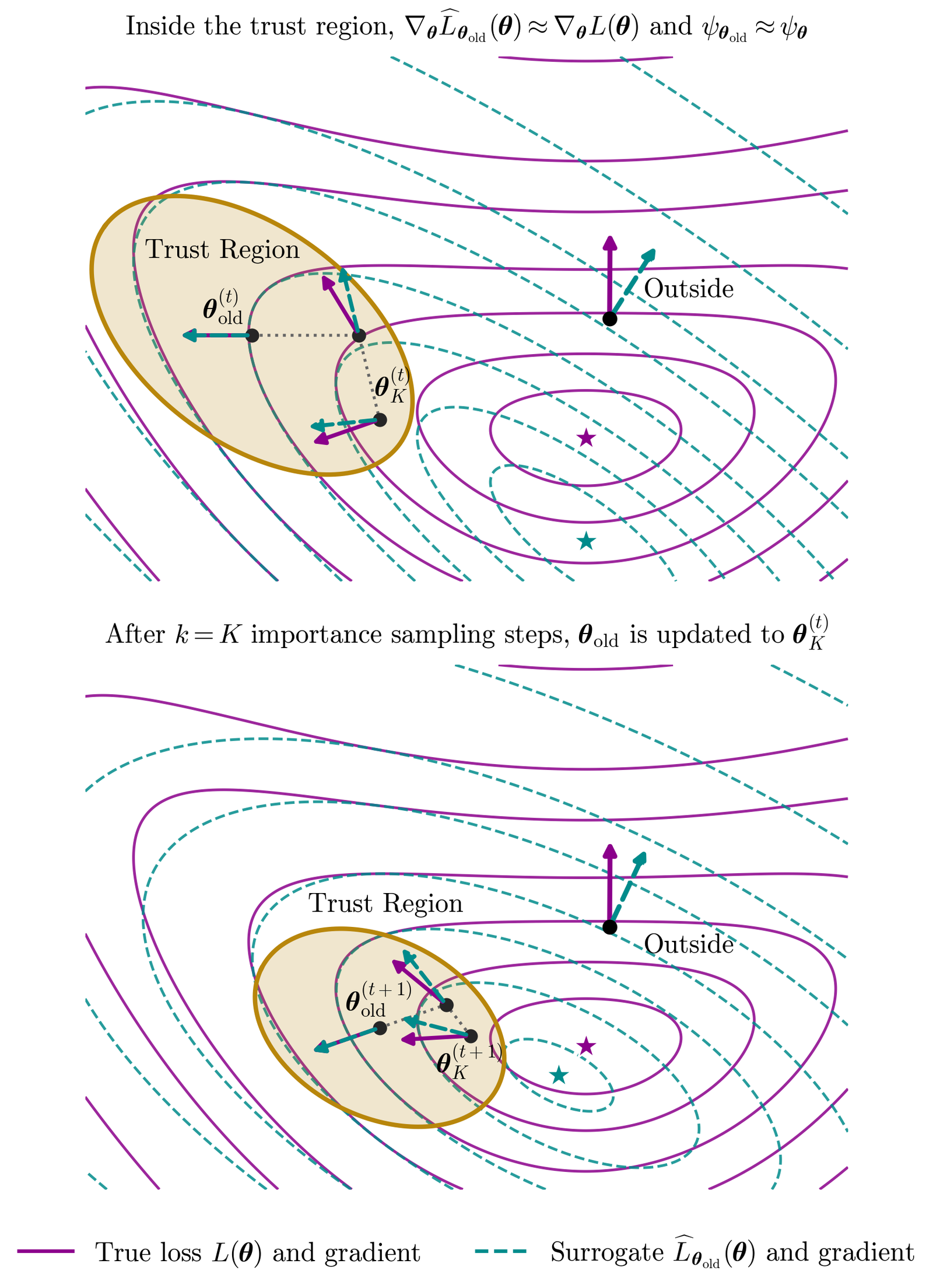
The resulting optimization procedure is summarized in Algorithm 1. The main differences from the original algorithm of SGD for VMC are the new loss function \(\overline{L}_{\mathrm{PWO}}(\vb*{\theta}; \vb*{\theta}_{\mathrm{old}})\) and the inclusion of an inner loop that performs multiple optimization steps using the cached samples from a previous parametrization of the wavefunction. This last point makes the average cost per optimization step of PWO significantly lower than other first- and second-order optimization methods for VMC, especially when samples are expensive to obtain or local energy evaluations are costly.
Example with NetKet
In this section, we provide a simple demo of how to use NetKet (Vicentini et al. 2022) to search for a low-energy neural quantum state with PWO. Since the optimal values of the hyperparameters are different for different initializations of the model, we fix one model initialization and run hyperparameter optimization (HPO) with Optuna. Every trial starts from the same variables and sampler seed, with a fresh optimizer and the same training-time budget. We then report the best trials using exact energy and variance evaluations, without retraining them.
This is a code example, not a comparison across optimizers. For such a comparison, we would repeat the entire HPO independently for each optimizer and each of several paired seeds, with matched search budgets. This simulates several people independently searching for a good solution with each method and lets us quantify variability across searches. Repeating the comparison over representative Hamiltonians, system sizes, lattice geometries, and architectures would test how broadly the conclusions apply.
A different question is which hyperparameter regions work well across initializations. To explore that question, we could draw a new initialization for every trial, obtaining noisy observations across seeds, or evaluate each configuration on several seeds and optimize its mean performance. The fixed-seed study below instead asks which configurations find the best state from this particular starting point.
Dependencies
For this demo, we need the following Python packages:
Next, we print the versions of these packages and the JAX device being used.
print("Python version:", sys.version)
print("NumPy version:", np.__version__)
print("Pandas version:", pd.__version__)
print("JAX version:", jax.__version__)
print("Optax version:", optax.__version__)
print("Flax version:", flax.__version__)
print("NetKet version:", nk.__version__)
print("Optuna version:", optuna.__version__)
print("JAX device:", jax.devices()[0])
Python version: 3.11.13 (main, Oct 7 2025, 15:34:32) [Clang 20.1.4 ]
NumPy version: 2.3.5
Pandas version: 3.0.1
JAX version: 0.9.0.1
Optax version: 0.2.6
Flax version: 0.12.4
NetKet version: 3.22.4
Optuna version: 5.0.0
JAX device: cuda:0Problem definition
The problem that we aim to solve is finding the ground-state energy of a 12-site periodic \(J_1\)-\(J_2\) Heisenberg chain with \(J_2/J_1=0.5\) (Majumdar-Ghosh point), whose Hamiltonian is: \[ \hat{\mathbf{H}} = J_1 \sum_{\langle i,j \rangle} \hat{\mathbf{S}}^{(i)} \cdot \hat{\mathbf{S}}^{(j)} + J_2 \sum_{\langle\langle i,j \rangle\rangle} \hat{\mathbf{S}}^{(i)} \cdot \hat{\mathbf{S}}^{(j)}, \] where \(\langle i,j \rangle\) denotes nearest-neighbor pairs and \(\langle\langle i,j \rangle\rangle\) denotes next-nearest-neighbor pairs. This is a prototypical example of a frustrated quantum spin system, where competing interactions prevent the system from easily settling into a simple ordered state. To make it more challenging, we choose not to apply the Marshall sign rule.
N = 12

graph = nk.graph.Chain(length=N, pbc=True, max_neighbor_order=2)
hilbert = nk.hilbert.Spin(s=0.5, N=N)
hamiltonian = nk.operator.Heisenberg(
    hilbert=hilbert,
    graph=graph,
    J=[1.0, 0.5],
    sign_rule=[False, False],
)
Since the problem is small enough, we can solve it exactly using full exact diagonalization to obtain the true ground-state energy and then compare it with the energy obtained from our NQS approximation:
eigenvalues = nk.exact.full_ed(hamiltonian)
E_true = eigenvalues[0]

print(f"Exact ground-state energy: {E_true:.8f}")
Exact ground-state energy: -18.00000000The ansatz we will employ is a compact autoregressive NQS based on a gated recurrent unit (GRU) backbone. The recurrent network processes the input configuration to produce contextual representations, which are passed through a shared nonlinear projection and two separate output heads. The amplitude head parameterizes normalized categorical conditionals through a log-softmax, while the phase head directly predicts bounded phase contributions using a scaled hyperbolic tangent. The resulting complex log-wavefunction combines the log-amplitude and phase contributions at each autoregressive position. For machine_pow = 2, the squared wavefunction amplitudes coincide with the normalized autoregressive probability distribution, ensuring normalization by construction.
class ComplexGRU(nk.models.AbstractARNN):
    hilbert: nk.hilbert.HomogeneousHilbert
    features: int = 64
    layers: int = 1
    head_hidden: int = 32
    machine_pow: int = 2

    @nn.compact
    def conditionals_log_psi(self, inputs):
        inputs = jnp.atleast_2d(inputs)
        hidden = inputs[..., None]
        for layer in range(self.layers):
            hidden = RNNLayer(
                cell=GRU1DCell(features=self.features, param_dtype=jnp.float32),
                exclusive=(layer == 0),
                name=f"gru_{layer}",
            )(hidden)

        hidden = nn.gelu(nn.Dense(self.head_hidden, name="shared_head")(hidden))

        amplitude_logits = nn.Dense(self.hilbert.local_size, name="amplitude")(hidden)
        log_amplitude = jax.nn.log_softmax(amplitude_logits, axis=-1) / self.machine_pow

        phase_logits = nn.Dense(
            self.hilbert.local_size,
            name="phase",
            kernel_init=nn.initializers.normal(stddev=1e-3),
        )(hidden)
        phase = jnp.pi * jnp.tanh(phase_logits)

        return log_amplitude + 1j * phase
We now instantiate the model with the specified number of features and layers.
LAYERS = 1
FEATURES = 64
HEAD_HIDDEN = 32

model = ComplexGRU(
    hilbert=hilbert,
    features=FEATURES,
    layers=LAYERS,
    head_hidden=HEAD_HIDDEN
)
Finally, we set up the sampler for the autoregressive model:
sampler = nk.sampler.ARDirectSampler(hilbert=hilbert)PWO driver
The next step is to define the loss function and the optimization driver for the PWO algorithm. The loss implements the modulus and phase surrogates introduced above:
def pwo_loss(
    params,
    batch: jax.Array,
    log_psi_old: jax.Array,
    adv_real: jax.Array,
    adv_imag: jax.Array,
    *,
    model,
    mod_clip_eps: float,
    arg_clip_eps: float,
    is_autoregressive: bool,
) -> jax.Array:

    log_psi_new = model.apply({"params": params}, batch)

    # Modulus channel:
    ratio = jnp.exp(2 * jnp.real(log_psi_new - log_psi_old))
    if not is_autoregressive:
        ratio = ratio / jax.lax.stop_gradient(jnp.mean(ratio))

    ratio_clip = jnp.clip(ratio, 1 - mod_clip_eps, 1 + mod_clip_eps)
    loss_mod = jnp.mean(jnp.maximum(ratio * adv_real, ratio_clip * adv_real))

    # Phase channel:
    sg_ratio = jax.lax.stop_gradient(ratio)
    phase_diff = jnp.imag(log_psi_new - log_psi_old)
    phase_diff = jnp.atan2(jnp.sin(phase_diff), jnp.cos(phase_diff))
    phi = 2 * phase_diff
    phi_clip = jnp.clip(phi, -arg_clip_eps, arg_clip_eps)
    loss_arg = jnp.mean(sg_ratio * jnp.maximum(phi * adv_imag, phi_clip * adv_imag))

    return loss_mod + loss_arg
The driver caches the samples, reference wavefunction, and centered local energies for is_steps updates before refreshing them:
class ProximalWavefunctionOptimization(nk.driver.AbstractOptimizationDriver):
    _ha: object = struct.field(pytree_node=False, serialize=False)
    _is_steps: int = struct.field(pytree_node=False)
    _batch: jax.Array | None = struct.field(default=None, serialize=False)
    _log_psi_old: jax.Array | None = struct.field(default=None, serialize=False)
    _adv_real: jax.Array | None = struct.field(default=None, serialize=False)
    _adv_imag: jax.Array | None = struct.field(default=None, serialize=False)
    _pwo_evaluate: object = struct.field(pytree_node=False, serialize=False)
    _pwo_loss: jax.Array | None = struct.field(default=None, serialize=False)

    def __init__(
        self,
        hamiltonian,
        optimizer,
        vstate: nk.vqs.MCState,
        *,
        is_steps: int = 4,
        mod_clip_eps: float = 0.2,
        arg_clip_eps: float = 0.2,
    ):

        super().__init__(vstate, optimizer, minimized_quantity_name="Energy")

        self._ha = hamiltonian
        self._is_steps = is_steps

        model = vstate.model
        is_autoregressive = isinstance(model, nk.models.AbstractARNN)
        self._pwo_evaluate = jax.jit(
            jax.value_and_grad(
                partial(
                    pwo_loss,
                    model=model,
                    mod_clip_eps=mod_clip_eps,
                    arg_clip_eps=arg_clip_eps,
                    is_autoregressive=is_autoregressive,
                )
            )
        )

    def _epoch_start(self) -> None:
        self.state.reset()
        self._batch = self.state.samples.reshape(-1, self.state.hilbert.size)
        self._log_psi_old = jax.lax.stop_gradient(self.state.log_value(self._batch))
        e_loc_chains = jax.lax.stop_gradient(self.state.local_estimators(self._ha))
        self._loss_stats = nk.stats.statistics(e_loc_chains)
        e_loc = e_loc_chains.reshape(-1)

        self._adv_real = jnp.real(e_loc) - jnp.mean(jnp.real(e_loc))
        self._adv_imag = jnp.imag(e_loc) - jnp.mean(jnp.imag(e_loc))

    def compute_loss_and_update(self):
        if self._batch is None or self.step_count % self._is_steps == 0:
            self._epoch_start()

        self._pwo_loss, grads = self._pwo_evaluate(
            self.state.parameters,
            self._batch,
            self._log_psi_old,
            self._adv_real,
            self._adv_imag,
        )

        return self._loss_stats, grads

    def _log_additional_data(self, log_dict: dict) -> None:
        log_dict["PWO_loss"] = self._pwo_loss
Training loop
For training, we will define a time budget instead of a fixed number of epochs. This makes a fair comparison between runs with different values of is_steps during the HPO: the total training time is kept constant, regardless of how frequently the PWO updates are applied. This would also be the way to make a consistent comparison of PWO with other optimization strategies like SR.
We will make use of a learning rate schedule based on cosine decay, which gradually reduces the learning rate from its initial value to a fraction of it over the course of the training time. Optax schedules operate based on the number of steps, but here we want to base it on the elapsed time relative to a fixed time budget. Therefore, we define a custom callback to this end.
class TimeCosineDecay(nk.callbacks.AbstractCallback):
    timeout: nk.callbacks.Timeout = struct.field(pytree_node=False)
    learning_rate: float = struct.field(pytree_node=False)
    alpha: float = struct.field(pytree_node=False)

    def __init__(self, timeout, learning_rate, alpha):
        super().__init__()
        self.timeout = timeout
        self.learning_rate = learning_rate
        self.alpha = alpha

    def before_parameter_update(self, step, log_data, driver):
        elapsed = time.time() - self.timeout._init_time
        fraction = np.clip(elapsed / self.timeout.timeout, 0.0, 1.0)
        rate = self.learning_rate * (
            self.alpha + 0.5 * (1 - self.alpha) * (1 + np.cos(np.pi * fraction))
        )
        hyperparams = driver._optimizer_state.hyperparams
        hyperparams["learning_rate"] = jnp.asarray(
            rate, dtype=hyperparams["learning_rate"].dtype
        )
Next, we define an auxiliary function to initialize the model, sampler, and variational state, and to run the PWO optimization with the specified time budget and learning rate schedule.
def run_pwo(
    hamiltonian,
    model,
    sampler,
    seed,
    sampler_seed,
    *,
    n_samples: int,
    training_time: float,
    alpha: float,
    learning_rate: float,
    mod_clip_eps: float = 0.2,
    arg_clip_eps: float = 0.2,
    is_steps: int = 4,
):
    vstate = nk.vqs.MCState(
        sampler=sampler,
        model=model,
        n_samples=n_samples,
        seed=seed,
        sampler_seed=sampler_seed,
    )
    optimizer = optax.inject_hyperparams(optax.adam)(learning_rate=learning_rate)
    driver = ProximalWavefunctionOptimization(
        hamiltonian=hamiltonian,
        optimizer=optimizer,
        vstate=vstate,
        is_steps=is_steps,
        mod_clip_eps=mod_clip_eps,
        arg_clip_eps=arg_clip_eps,
    )
    logger = nk.logging.RuntimeLog()
    timeout = nk.callbacks.Timeout(training_time)

    driver.run(
        n_iter=1_000_000_000,
        out=logger,
        show_progress=False,
        callback=[TimeCosineDecay(timeout, learning_rate, alpha), timeout],
    )

    return vstate, logger
HPO
For the hyperparameter optimization, we will use the exact final variational energy as the objective. Exact summation is affordable for this small system and avoids selecting a trial because of a favorable Monte Carlo estimate. If exact summation was not affordable, one could increase the number of Monte Carlo samples for final evaluation of each run to reduce the statistical error and make the selection more reliable. Variance and relative error are also recorded as diagnostics, but not as additional selection objectives.
def fullsum_energy(hamiltonian, vstate):
    fullsum_state = nk.vqs.FullSumState(
        hilbert=vstate.hilbert,
        model=vstate.model,
        variables=vstate.variables,
    )
    energy = fullsum_state.expect(hamiltonian)

    return energy

def relative_error(y_pred, y_true):
    return (y_pred - y_true) / jnp.abs(y_true)
In order to perform hyperparameter optimization, we define a function that suggests hyperparameters based on a trial object and a predefined configuration:
def suggest_hyperparameter(trial: optuna.trial.BaseTrial, name: str, config: dict):
    parameter_type = config["type"]
    if parameter_type == "categorical":
        suggestion = trial.suggest_categorical(name, config["choices"])
    elif parameter_type == "float":
        suggestion = trial.suggest_float(
            name,
            float(config["low"]),
            float(config["high"]),
            step=config.get("step"),
            log=config.get("log", False),
        )
    elif parameter_type == "int":
        suggestion = trial.suggest_int(
            name,
            int(config["low"]),
            int(config["high"]),
            step=int(config["step"]) if config.get("step") is not None else 1,
            log=config.get("log", False),
        )
    else:
        raise ValueError(f"Unknown parameter type: {parameter_type}")

    return suggestion
The hyperparameter search space is defined in the HPO_SUGGESTIONS dictionary, where each entry specifies the type of the hyperparameter and its corresponding range or choices. The suggest_hyperparameter function uses this configuration to suggest values for each hyperparameter during the optimization process.
HPO_SUGGESTIONS = {
    "learning_rate": {"type": "float", "low": 1e-5, "high": 1e-1, "log": True},
    "alpha": {"type": "float", "low": 0.01, "high": 0.5, "log": True},
    "mod_clip_eps": {"type": "float", "low": 1e-5, "high": 1.0, "log": True},
    "arg_clip_eps": {"type": "float", "low": 1e-5, "high": np.pi, "log": True},
    "is_steps": {"type": "int", "low": 1, "high": 8},
}
The search includes is_steps=1: refreshing the reference before every update recovers the ordinary VMC gradient, optimized here with Adam. Note that the positive clipping thresholds do not affect this no-reuse ablation. In theory, this would tell us whether reusing the reference provides a genuine advantage. However, a finite HPO cannot guarantee that either variant is optimally tuned.
In the following cell, we define the objective function for the HPO, which runs the PWO algorithm with the suggested hyperparameters and evaluates the resulting variational state using exact summation. Each call to run_pwo uses the same initialization and sampler seeds, reproducing the same starting state.
ROOT_SEED = 1234
INIT_KEY, SAMPLER_KEY = jax.random.split(jax.random.key(ROOT_SEED))
N_SAMPLES = 1024
TRAINING_TIME = 60.0

def objective(trial: optuna.trial.BaseTrial):
    suggestions = {
        name: suggest_hyperparameter(trial, name, config)
        for name, config in HPO_SUGGESTIONS.items()
    }
    vstate, _ = run_pwo(
        hamiltonian=hamiltonian,
        model=model,
        sampler=sampler,
        seed=INIT_KEY,
        sampler_seed=SAMPLER_KEY,
        n_samples=N_SAMPLES,
        training_time=TRAINING_TIME,
        **suggestions,
    )
    stats = fullsum_energy(hamiltonian, vstate)
    energy = float(np.real(stats.mean))
    metrics = {
        "exact_energy": energy,
        "absolute_error": energy - E_true,
        "relative_error": float(relative_error(energy, E_true)),
        "exact_variance": float(stats.variance),
    }
    if not np.all(np.isfinite(list(metrics.values()))):
        return float("nan")

    for name, value in metrics.items():
        trial.set_user_attr(name, value)

    return energy
Finally, we create an Optuna study and run the hyperparameter optimization for a specified number of trials. The study uses a TPE sampler with a fixed seed to ensure reproducibility.
HPO_SEED = ROOT_SEED + 1
N_HPO_TRIALS = 100

study = optuna.create_study(
    direction="minimize",
    sampler=optuna.samplers.TPESampler(seed=HPO_SEED),
)
study.optimize(objective, n_trials=N_HPO_TRIALS)
Results
The following table ranks the best 5 completed trials by exact energy and includes their absolute and relative errors, variance, and hyperparameters. These are the actual trial endpoints, not new runs with the selected settings. They are selected configurations for one initialization, not independent replications.
Code
N_BEST = 5

completed_trials = [
    trial for trial in study.trials
    if trial.state == optuna.trial.TrialState.COMPLETE
    and trial.value is not None and np.isfinite(trial.value)
]

print(f"Completed trials: {len(completed_trials)}/{len(study.trials)}")

best_trials = sorted(completed_trials, key=lambda trial: (trial.value, trial.number))[:N_BEST]
results = pd.DataFrame([
    {"trial": trial.number, **trial.user_attrs, **trial.params}
    for trial in best_trials
])
results.index = pd.RangeIndex(1, len(results) + 1, name="rank")
formats = {name: "{:.6g}" for name in results.columns if name not in ("trial", "is_steps")}
display(results.style.format(formats))
Completed trials: 100/100| trial | exact_energy | absolute_error | relative_error | exact_variance | learning_rate | alpha | mod_clip_eps | arg_clip_eps | is_steps | |
|---|---|---|---|---|---|---|---|---|---|---|
| rank | ||||||||||
| 1 | 87 | -17.9999 | 5.25982e-05 | 2.92212e-06 | 0.000409964 | 0.013136 | 0.0320371 | 0.000793604 | 0.00190924 | 3 |
| 2 | 70 | -17.9999 | 7.49249e-05 | 4.1625e-06 | 0.000654246 | 0.0142461 | 0.0259956 | 0.000692447 | 0.000510366 | 3 |
| 3 | 58 | -17.9999 | 0.000103218 | 5.73436e-06 | 0.00118784 | 0.0105194 | 0.0311586 | 0.000589571 | 0.00377736 | 4 |
| 4 | 9 | -17.9998 | 0.000151157 | 8.3976e-06 | 0.00111878 | 0.000932078 | 0.0192634 | 0.57069 | 1.84929 | 5 |
| 5 | 90 | -17.9998 | 0.000192986 | 1.07214e-05 | 0.00226042 | 0.00950345 | 0.0334082 | 0.00121769 | 0.000737893 | 3 |
We can also visualize the optimization history and the explored hyperparameter configurations using Optuna’s built-in plotting functions. Remember that these visualizations reflect the performance observed in this fixed-seed study and do not necessarily indicate universally optimal hyperparameter settings. First, in Figure 4, we show the optimization history:
Code
fig = optuna.visualization.plot_optimization_history(
    study,
    target_name="Variational energy",
    )
fig.update_layout(
    template="science",
    title=None,
    showlegend=False,
)

show_plotly(fig)The second plot, in Figure 5, shows the parallel coordinate plot of the explored hyperparameter configurations, colored by the variational energy:
Code
from plotly.colors import sample_colorscale

fig = optuna.visualization.plot_parallel_coordinate(
    study,
    target_name="Variational energy",
)

completed_trials = sorted(
    (
        trial for trial in study.trials
        if trial.state == optuna.trial.TrialState.COMPLETE and trial.value is not None
    ),
    key=lambda trial: trial.number,
)
energies = np.array([trial.value for trial in completed_trials], dtype=float)
energy_min, energy_max = float(energies.min()), float(energies.max())
normalized_energies = (energies - energy_min) / (energy_max - energy_min)
energy_colorscale = "Agsunset"
trial_colors = sample_colorscale(energy_colorscale, normalized_energies.tolist())
line_traces = [trace for trace in fig.data if trace.mode == "lines"]
for trace, color, trial in zip(line_traces, trial_colors, completed_trials, strict=True):
    trace.line.color = color
    trace.line.shape = "spline"
    trial_parameters = "<br>".join(
        f"{name}: {value:.6g}" if isinstance(value, (int, float)) else f"{name}: {value}"
        for name, value in trial.params.items()
    )
    trace.hovertemplate = (
        f"Trial {trial.number}<br>"
        f"Variational energy: {trial.value:.6g}<br>"
        f"{trial_parameters}<extra></extra>"
    )

colorbar_trace = next(trace for trace in fig.data if trace.marker.showscale)
colorbar_trace.marker.update(
    color=[energy_min, energy_max],
    colorscale=energy_colorscale,
    cmin=energy_min,
    cmax=energy_max,
    reversescale=False,
    colorbar=dict(
        title=dict(text="Variational energy", side="right"),
        thickness=14,
    ),
)
fig.update_layout(
    template="science",
    title=None,
    margin=dict(l=10),
)
show_plotly(fig)The third plot, in Figure 6, shows the pairwise relationships between hyperparameters and the variational energy, providing insight into potential interactions and dependencies:
Code
fig = optuna.visualization.plot_contour(
    study,
    target_name="Variational energy",
)
fig.update_traces(
    colorscale=energy_colorscale,
            reversescale=False,
    colorbar=dict(
        title=dict(text="Variational energy", side="right"),
        thickness=14,
    ),
    selector=dict(type="contour"),
        )
fig.update_layout(template="science", title=None, height=750)
show_plotly(fig)Finally, Figure 7 shows the estimated importance of each hyperparameter for the variational energy objective. Take into account that the clipping thresholds are inactive when is_steps=1, which can affect their estimated importance.
Code
fig = optuna.visualization.plot_param_importances(
    study,
    target_name="Variational energy",
)
fig.update_traces(textposition="none", selector=dict(type="bar"))
fig.update_layout(template="science", title=None)
fig.update_yaxes(tickangle=45)
show_plotly(fig)Conclusions
Neural Quantum States (NQS) are a powerful ansatz for representing quantum many-body wavefunctions, but their optimization is currently limited due to:
- The potentially poor sample efficiency of MCMC methods and the fact that samples are discarded after each update.
- The fact that SR can be ill-conditioned, specially for AR models, and scales poorly with the number of parameters and samples.
Proximal Wavefunction Optimization (PWO) is a scalable first-order optimization method for NQS, derived from an explicit connection between VMC and RL, that resembles PPO. This method is computationally cheaper than SGD and minSR, allows for sample reuse across optimization steps and provides the convergence stability of higher order methods via a trust region in wavefunction space. The proposed algorithm is supported by both theoretical and empirical evidence. More broadly, this work bridges the RL and NQS communities, enabling further mutual inspiration.
Appendix
Auxiliary results
Let \(\ket{\psi_{\boldsymbol{\theta}}}\) and \(\ket{\psi_{\boldsymbol{\theta}'}}\) be normalized wavefunctions, and choose the global phase of \(\ket{\psi_{\boldsymbol{\theta}'}}\) so that \[ \braket{\psi_{\boldsymbol{\theta}}}{\psi_{\boldsymbol{\theta}'}} = \abs{\braket{\psi_{\boldsymbol{\theta}}}{\psi_{\boldsymbol{\theta}'}}} = \sqrt{1-\mathcal I(\psi_{\boldsymbol{\theta}},\psi_{\boldsymbol{\theta}'})}, \tag{2}\] where \(\mathcal I(\psi_{\boldsymbol{\theta}},\psi_{\boldsymbol{\theta}'})\) denotes the infidelity between the two wavefunctions. Define \[ r_{\boldsymbol{\theta}';\boldsymbol{\theta}}(\vb{s}) := \frac{\mathcal P_{\boldsymbol{\theta}'}(\vb{s})}{\mathcal P_{\boldsymbol{\theta}}(\vb{s})}\qq{and} z_{\boldsymbol{\theta}';\boldsymbol{\theta}}(\vb{s}) := \frac{\psi_{\boldsymbol{\theta}'}(\vb{s})}{\psi_{\boldsymbol{\theta}}(\vb{s})}. \] We write \(z_{\boldsymbol{\theta}';\boldsymbol{\theta}}=\sqrt{r_{\boldsymbol{\theta}';\boldsymbol{\theta}}}e^{i\alpha_{\boldsymbol{\theta}';\boldsymbol{\theta}}}\), where \[ \alpha_{\boldsymbol{\theta}';\boldsymbol{\theta}}(\vb{s}) = \atan_2\!\left( \sin\!\left(\arg\psi_{\boldsymbol{\theta}'}(\vb{s})-\arg\psi_{\boldsymbol{\theta}}(\vb{s})\right), \cos\!\left(\arg\psi_{\boldsymbol{\theta}'}(\vb{s})-\arg\psi_{\boldsymbol{\theta}}(\vb{s})\right) \right), \] and \(\phi_{\boldsymbol{\theta}';\boldsymbol{\theta}}=2\alpha_{\boldsymbol{\theta}';\boldsymbol{\theta}}\).
Theorem 1 Let \(\hat K_{\boldsymbol{\theta}}=\hat H-E[\psi_{\boldsymbol{\theta}}]\I\). Then \[ E[\psi_{\boldsymbol{\theta}'}]-E[\psi_{\boldsymbol{\theta}}] = 2\Re\Bqty{ \E_{\mathcal P_{\boldsymbol{\theta}}} \left[ z_{\boldsymbol{\theta}';\boldsymbol{\theta}}^* \Delta E^{\mathrm{loc}}_{\boldsymbol{\theta}} \right]} + \mel{\eta}{\hat K_{\boldsymbol{\theta}}}{\eta}, \tag{3}\] where \(\ket{\eta}=\ket{\psi_{\boldsymbol{\theta}'}}-\ket{\psi_{\boldsymbol{\theta}}}\). Consequently, \[ \begin{aligned} E[\psi_{\boldsymbol{\theta}'}]-E[\psi_{\boldsymbol{\theta}}] \leq{}& 2\E_{\mathcal P_{\boldsymbol{\theta}}} \left[ \sqrt{r_{\boldsymbol{\theta}';\boldsymbol{\theta}}} \cos\alpha_{\boldsymbol{\theta}';\boldsymbol{\theta}} A_{\vb*{\theta}}^{\mathrm{R}} \right]\\ &+ 2\E_{\mathcal P_{\boldsymbol{\theta}}} \left[ \sqrt{r_{\boldsymbol{\theta}';\boldsymbol{\theta}}} \sin\alpha_{\boldsymbol{\theta}';\boldsymbol{\theta}} A_{\vb*{\theta}}^{\mathrm{I}} \right] \nonumber\\ &+ 2\norm{\hat H-E[\psi_{\boldsymbol{\theta}}]\I}_{\infty} \left(1-\sqrt{1-\mathcal I(\psi_{\boldsymbol{\theta}},\psi_{\boldsymbol{\theta}'})}\right). \label{eq:exact-complex-upper-bound} \end{aligned} \tag{4}\]
Proof. Expanding around the reference state gives \[ E[\psi_{\boldsymbol{\theta}'}]-E[\psi_{\boldsymbol{\theta}}] = \mel{\psi_{\boldsymbol{\theta}'}}{\hat K_{\boldsymbol{\theta}}}{\psi_{\boldsymbol{\theta}'}} = 2\Re\mel{\eta}{\hat K_{\boldsymbol{\theta}}}{\psi_{\boldsymbol{\theta}}} + \mel{\eta}{\hat K_{\boldsymbol{\theta}}}{\eta}. \] Since \(\eta(\vb{s})=(z_{\boldsymbol{\theta}';\boldsymbol{\theta}}(\vb{s})-1)\psi_{\boldsymbol{\theta}}(\vb{s})\) and \(\mel{\vb{s}}{\hat K_{\boldsymbol{\theta}}}{\psi_{\boldsymbol{\theta}}}=\psi_{\boldsymbol{\theta}}(\vb{s})\Delta E^{\mathrm{loc}}_{\boldsymbol{\theta}}(\vb{s})\), \[ \mel{\eta}{\hat K_{\boldsymbol{\theta}}}{\psi_{\boldsymbol{\theta}}} = \E_{\mathcal P_{\boldsymbol{\theta}}} \left[(z_{\boldsymbol{\theta}';\boldsymbol{\theta}}^*-1)\Delta E^{\mathrm{loc}}_{\boldsymbol{\theta}}\right] = \E_{\mathcal P_{\boldsymbol{\theta}}} \left[z_{\boldsymbol{\theta}';\boldsymbol{\theta}}^*\Delta E^{\mathrm{loc}}_{\boldsymbol{\theta}}\right], \] because \(\E_{\mathcal P_{\boldsymbol{\theta}}}[\Delta E^{\mathrm{loc}}_{\boldsymbol{\theta}}]=0\). According to Cauchy-Schwarz inequality, the remainder satisfies \[ \mel{\eta}{ \hat K_{\boldsymbol{\theta}} }{ \eta } \leq \abs{ \mel{\eta}{ \hat K_{\boldsymbol{\theta}} }{ \eta } }\leq \norm{\eta}\norm{\hat{K}_{\boldsymbol{\theta}}\ket{\eta}} \leq \norm{\eta}\norm{\hat{K}_{\boldsymbol{\theta}}}_\infty\norm{\eta} = \left\| \hat K_{\boldsymbol{\theta}} \right\|_\infty \|\eta\|^2, \] with \[ \norm{\eta}^2=2- 2\Re \braket{ \psi_{\boldsymbol{\theta}} }{ \psi_{\boldsymbol{\theta}'} }=2\left(1-\sqrt{1-\mathcal I(\psi_{\boldsymbol{\theta}},\psi_{\boldsymbol{\theta}'})}\right), \] where we have used the global-phase convention in Equation 2. Finally, \[ \Re \left[ z_{\boldsymbol{\theta}';\boldsymbol{\theta}}^* \Delta E^{\mathrm{loc}}_{\boldsymbol{\theta}} \right] = \sqrt{r_{\boldsymbol{\theta}';\boldsymbol{\theta}}} \left( \cos\alpha_{\boldsymbol{\theta}';\boldsymbol{\theta}}A_{\vb*{\theta}}^{\mathrm{R}} + \sin\alpha_{\boldsymbol{\theta}';\boldsymbol{\theta}}A_{\vb*{\theta}}^{\mathrm{I}} \right), \] which proves the desired inequality.
Lemma 1 For every \(t\geq0\) and \(\alpha\in[-\pi,\pi]\), \[ \abs{2t\sin\alpha-2t^2\alpha} \leq 4\pi^2\abs{te^{i\alpha}-1}^2. \tag{5}\]
Proof. Set \[ d(t,\alpha) := \abs{te^{i\alpha}-1}^2 = (t-1)^2+2t(1-\cos\alpha). \] We distinguish three ranges of \(t\).
Case 1: \(0\leq t\leq 1/2\).
Using \(\abs{\sin\alpha}\leq1\) and \(\abs{\alpha}\leq\pi\), we obtain \[ \abs{2t\sin\alpha-2t^2\alpha} \leq 2t+2\pi t^2 \leq 1+\frac{\pi}{2}. \] On the other hand, \[ d(t,\alpha)\geq(1-t)^2\geq\frac14. \] Hence \[ \abs{2t\sin\alpha-2t^2\alpha} \leq (4+2\pi)d(t,\alpha) \leq 4\pi^2d(t,\alpha). \]
Case 2: \(t\geq2\).
Again, \[ \abs{2t\sin\alpha-2t^2\alpha} \leq 2t+2\pi t^2. \] Since \(t-1\geq t/2\), we have \[ d(t,\alpha)\geq(t-1)^2\geq\frac{t^2}{4}. \] It follows that \[ \abs{2t\sin\alpha-2t^2\alpha} \leq \left( \frac{8}{t}+8\pi \right)d(t,\alpha) \leq (4+8\pi)d(t,\alpha) \leq 4\pi^2d(t,\alpha). \]
Case 3: \(1/2\leq t\leq2\).
We first separate the error caused by replacing \(\sin\alpha\) with \(\alpha\) from the error caused by replacing \(t\) with \(t^2\): \[\begin{align} 2t\sin\alpha-2t^2\alpha &= 2t(\sin\alpha-\alpha) + 2t\alpha(1-t). \end{align}\] Therefore, \[ \abs{2t\sin\alpha-2t^2\alpha} \leq 2t\abs{\sin\alpha-\alpha} + 2t\abs{\alpha}\abs{1-t} \leq t\alpha^2 + 2t\abs{\alpha}\abs{1-t}, \tag{6}\] where we used the elementary Taylor bound \(\abs{\sin\alpha-\alpha}\leq \alpha^2/2\). For \(\alpha\in[-\pi,\pi]\), we also have \(1-\cos\alpha\geq 2\alpha^2/\pi^2\). Consequently, \[ d(t,\alpha) \geq (t-1)^2+\frac{4t\alpha^2}{\pi^2}. \tag{7}\] The second term on the right-hand side immediately gives \[ t\alpha^2 \leq \frac{\pi^2}{4}d(t,\alpha). \tag{8}\]
To control the mixed term, define \[ x:=\abs{1-t}, \qquad y:=\frac{2\sqrt{t}\abs{\alpha}}{\pi}. \] Then Equation 7 says that \[ d(t,\alpha)\geq x^2+y^2, \] while \[ 2t\abs{\alpha}\abs{1-t} = \pi\sqrt{t}\,xy. \] Using \(2xy\leq x^2+y^2\) and \(t\leq2\), we obtain \[ 2t\abs{\alpha}\abs{1-t} \leq \frac{\pi\sqrt{t}}{2}(x^2+y^2) \leq \frac{\pi\sqrt{2}}{2}d(t,\alpha). \tag{9}\] Combining Equation 6, Equation 8, and Equation 9, we find \[ \abs{2t\sin\alpha-2t^2\alpha} \leq \left( \frac{\pi^2}{4} + \frac{\pi\sqrt{2}}{2} \right)d(t,\alpha) \leq 4\pi^2d(t,\alpha). \]
The three cases cover all \(t\geq0\), which proves Equation 5.
Define the unclipped PWO surrogates \[ S_{\mathrm{mod}}(\boldsymbol{\theta}';\boldsymbol{\theta}) = \E_{\mathcal P_{\boldsymbol{\theta}}} \left[ r_{\boldsymbol{\theta}';\boldsymbol{\theta}}A_{\vb*{\theta}}^{\mathrm{R}} \right], \tag{10}\] and \[ S_{\mathrm{arg}}(\boldsymbol{\theta}';\boldsymbol{\theta}) = \E_{\mathcal P_{\boldsymbol{\theta}}} \left[ r_{\boldsymbol{\theta}';\boldsymbol{\theta}} \phi_{\boldsymbol{\theta}';\boldsymbol{\theta}}A_{\vb*{\theta}}^{\mathrm{I}} \right]. \tag{11}\]
Theorem 2 Assume \(A_{\vb*{\theta}}^{\mathrm{R}}\) and \(A_{\vb*{\theta}}^{\mathrm{I}}\) are bounded. Then \[ \begin{aligned} E[\psi_{\boldsymbol{\theta}'}]-E[\psi_{\boldsymbol{\theta}}] \leq & S_{\mathrm{mod}}(\boldsymbol{\theta}';\boldsymbol{\theta}) + S_{\mathrm{arg}}(\boldsymbol{\theta}';\boldsymbol{\theta}) \\ &+ C_{\boldsymbol{\theta}} \left(1-\sqrt{1-\mathcal I(\psi_{\boldsymbol{\theta}},\psi_{\boldsymbol{\theta}'})}\right), \end{aligned} \tag{12}\] where one may take \[ C_{\boldsymbol{\theta}} = 2\pqty{\norm{\hat H-E[\psi_{\boldsymbol{\theta}}]\I}_{\infty} + \norm{A_{\vb*{\theta}}^{\mathrm{R}}}_{\infty} +4\pi^2\norm{A_{\vb*{\theta}}^{\mathrm{I}}}_{\infty}}. \tag{13}\] In particular, \[ E[\psi_{\boldsymbol{\theta}'}]-E[\psi_{\boldsymbol{\theta}}] \leq S_{\mathrm{mod}}(\boldsymbol{\theta}';\boldsymbol{\theta}) + S_{\mathrm{arg}}(\boldsymbol{\theta}';\boldsymbol{\theta}) + C_{\boldsymbol{\theta}} \mathcal I(\psi_{\boldsymbol{\theta}},\psi_{\boldsymbol{\theta}'}). \tag{14}\]
Proof. Write \(r\equiv r_{\boldsymbol{\theta}';\boldsymbol{\theta}}\), \(\alpha\equiv\alpha_{\boldsymbol{\theta}';\boldsymbol{\theta}}\), \(\phi\equiv 2\alpha\), and \(z\equiv\sqrt r e^{i\alpha}\). Since \(\abs{z-1}^2=1+r-2\sqrt r\cos\alpha\) and \(\E[A_{\vb*{\theta}}^{\mathrm{R}}]=0\), \[ 2\E_{\mathcal P_{\boldsymbol{\theta}}}[\sqrt r\cos\alpha A_{\vb*{\theta}}^{\mathrm{R}}] = \E_{\mathcal P_{\boldsymbol{\theta}}}[rA_{\vb*{\theta}}^{\mathrm{R}}]-\E_{\mathcal P_{\boldsymbol{\theta}}}[\abs{z-1}^2A_{\vb*{\theta}}^{\mathrm{R}}] \leq S_{\mathrm{mod}}+\norm{A_{\vb*{\theta}}^{\mathrm{R}}}_{\infty}\E_{\mathcal P_{\boldsymbol{\theta}}}[\abs{z-1}^2]. \] For the phase term, Lemma 1 with \(t=\sqrt r\) gives \[ \begin{aligned} 2\E_{\mathcal P_{\boldsymbol{\theta}}} \left[ \sqrt r\sin\alpha A_{\vb*{\theta}}^{\mathrm{I}} \right] &= \E_{\mathcal P_{\boldsymbol{\theta}}} \left[ 2 r\alpha\,A_{\vb*{\theta}}^{\mathrm{I}} \right] + \E_{\mathcal P_{\boldsymbol{\theta}}} \left[ \pqty{2\sqrt r\sin\alpha - 2r\alpha}A_{\vb*{\theta}}^{\mathrm{I}} \right]\nonumber\\ &\leq \E_{\mathcal P_{\boldsymbol{\theta}}} \left[ r\phi A_{\vb*{\theta}}^{\mathrm{I}} \right] + \E_{\mathcal P_{\boldsymbol{\theta}}} \left[\abs{2\sqrt r\sin\alpha - 2r\alpha}\abs{A_{\vb*{\theta}}^{\mathrm{I}}} \right]\nonumber\\ & \leq \E_{\mathcal P_{\boldsymbol{\theta}}}[r\phi A_{\vb*{\theta}}^{\mathrm{I}}] + 4\pi^2\norm{A_{\vb*{\theta}}^{\mathrm{I}}}_{\infty}\E_{\mathcal P_{\boldsymbol{\theta}}}[\abs{z-1}^2]\nonumber\\ & = S_{\mathrm{arg}}+4\pi^2\norm{A_{\vb*{\theta}}^{\mathrm{I}}}_{\infty}\E_{\mathcal P_{\boldsymbol{\theta}}}[\abs{z-1}^2]. \end{aligned} \] Finally, \[ \E_{\mathcal P_{\boldsymbol{\theta}}}[\abs{z-1}^2] = \norm{\psi_{\boldsymbol{\theta}'}-\psi_{\boldsymbol{\theta}}}^2 = 2\left(1-\sqrt{1-\mathcal I(\psi_{\boldsymbol{\theta}},\psi_{\boldsymbol{\theta}'})}\right). \] Combining these estimates with Theorem 1 proves Equation 12. The linear-infidelity form follows from \(1-\sqrt{1-x}\leq x\).
Theorem 3 Assume \(\psi_{\boldsymbol{\theta}}\) is differentiable in a neighborhood of the reference parameters and detach the importance sampling ratio from the gradient computation of the phase surrogate objective, i.e. make \(S_{\mathrm{arg}}(\boldsymbol{\theta}';\boldsymbol{\theta})= \E_{\mathcal P_{\boldsymbol{\theta}}}\left[\operatorname{sg}(r_{\boldsymbol{\theta}';\boldsymbol{\theta}})\phi_{\boldsymbol{\theta}';\boldsymbol{\theta}}A_{\vb*{\theta}}^{\mathrm{I}}\right]\). Then \[ \eval{\grad_{\boldsymbol{\theta}'} \left[ S_{\mathrm{mod}}(\boldsymbol{\theta}';\boldsymbol{\theta}) + S_{\mathrm{arg}}(\boldsymbol{\theta}';\boldsymbol{\theta}) \right]}_{\boldsymbol{\theta}'=\boldsymbol{\theta}} = \eval{\grad_{\boldsymbol{\theta}'}E[\psi_{\boldsymbol{\theta}'}]}_{\boldsymbol{\theta}'=\boldsymbol{\theta}}. \tag{15}\]
Proof. At \(\boldsymbol{\theta}'=\boldsymbol{\theta}\), \[ \left.\grad_{\boldsymbol{\theta}'}r_{\boldsymbol{\theta}';\boldsymbol{\theta}}(\vb{s})\right|_{\boldsymbol{\theta}'=\boldsymbol{\theta}} = \grad_{\boldsymbol{\theta}}\log\mathcal P_{\boldsymbol{\theta}}(\vb{s}) = 2\grad_{\boldsymbol{\theta}}\log\abs{\psi_{\boldsymbol{\theta}}(\vb{s})}, \] and \[ \left.\grad_{\boldsymbol{\theta}'}\phi_{\boldsymbol{\theta}';\boldsymbol{\theta}}(\vb{s})\right|_{\boldsymbol{\theta}'=\boldsymbol{\theta}} = 2\grad_{\boldsymbol{\theta}}\arg\psi_{\boldsymbol{\theta}}(\vb{s}). \] Thus the gradients of \(S_{\mathrm{mod}}\) and \(S_{\mathrm{arg}}\) recover the two terms in the VMC gradient Equation 1.
References
Agarwal, Alekh, Kiante Brantley, Nan Jiang, Sham M Kakade, and Wen Sun. n.d. Reinforcement Learning: Theory and Algorithms.
Amari, Shun-ichi. 1998. “Natural Gradient Works Efficiently in Learning.” Neural Computation 10 (2): 251–76. https://doi.org/10.1162/089976698300017746.
Baydin, Atilim Gunes, Barak A. Pearlmutter, Alexey Andreyevich Radul, and Jeffrey Mark Siskind. 2018. “Automatic Differentiation in Machine Learning: A Survey.” Journal of Machine Learning Research 18 (153): 1–43.
Becca, Federico, and Sandro Sorella. 2017. Quantum Monte Carlo Approaches for Correlated Systems. 1st ed. Cambridge University Press. https://doi.org/10.1017/9781316417041.
Bottou, Léon, Frank E. Curtis, and Jorge Nocedal. 2018. “Optimization Methods for Large-Scale Machine Learning.” SIAM Review 60 (2): 223–311. https://doi.org/10.1137/16M1080173.
Bronstein, Michael M., Joan Bruna, Taco Cohen, and Petar Veličković. 2021. Geometric Deep Learning: Grids, Groups, Graphs, Geodesics, and Gauges. arXiv:2104.13478. arXiv. https://doi.org/10.48550/arXiv.2104.13478.
Bronstein, Michael M., Joan Bruna, Yann LeCun, Arthur Szlam, and Pierre Vandergheynst. 2017. “Geometric Deep Learning: Going Beyond Euclidean Data.” IEEE Signal Processing Magazine 34 (4): 18–42. https://doi.org/10.1109/MSP.2017.2693418.
Carleo, Giuseppe, and Matthias Troyer. 2017. “Solving the Quantum Many-Body Problem with Artificial Neural Networks.” Science 355 (6325): 602–6. https://doi.org/10.1126/science.aag2302.
Chen, Ao, and Markus Heyl. 2024. “Empowering Deep Neural Quantum States Through Efficient Optimization.” Nature Physics 20 (9): 1476–81. https://doi.org/10.1038/s41567-024-02566-1.
Dawid, Anna. 2025. Machine Learning in Quantum Sciences. Cambridge University Press. https://doi.org/10.1017/9781009504942.
Del Debbio, Luigi, Gian Mario Manca, and Ettore Vicari. 2004. “Critical Slowing down of Topological Modes.” Physics Letters B 594 (3-4): 315–23. https://doi.org/10.1016/j.physletb.2004.05.038.
Deng, Dong-Ling, Xiaopeng Li, and S. Das Sarma. 2017. “Quantum Entanglement in Neural Network States.” Physical Review X 7 (2): 021021. https://doi.org/10.1103/PhysRevX.7.021021.
Goldshlager, Gil, Nilin Abrahamsen, and Lin Lin. 2024. “A Kaczmarz-Inspired Approach to Accelerate the Optimization of Neural Network Wavefunctions.” Journal of Computational Physics 516 (November): 113351. https://doi.org/10.1016/j.jcp.2024.113351.
Graesser, Laura, and Wah Loon Keng. 2020. Foundations of Deep Reinforcement Learning: Theory and Practice in Python. Addison Wesley Data & Analytics Series. Addison-Wesley.
Hastings, W. K. 1970. “Monte Carlo Sampling Methods Using Markov Chains and Their Applications.” Biometrika 57 (1): 97–109. https://doi.org/10.1093/biomet/57.1.97.
Hibat-Allah, Mohamed, Martin Ganahl, Lauren E. Hayward, Roger G. Melko, and Juan Carrasquilla. 2020. “Recurrent Neural Network Wave Functions.” Physical Review Research 2 (2): 023358. https://doi.org/10.1103/PhysRevResearch.2.023358.
Hornik, Kurt, Maxwell Stinchcombe, and Halbert White. 1989. “Multilayer Feedforward Networks Are Universal Approximators.” Neural Networks 2 (5): 359–66. https://doi.org/10.1016/0893-6080(89)90020-8.
Kakade, Sham M. 2001. “A Natural Policy Gradient.” Advances in Neural Information Processing Systems 14.
Kakade, Sham, and John Langford. 2002. “Approximately Optimal Approximate Reinforcement Learning.” Proceedings of the Nineteenth International Conference on Machine Learning (San Francisco, CA, USA), Icml ’02, 267–74.
Kingma, Diederik P., and Jimmy Ba. 2017. Adam: A Method for Stochastic Optimization. arXiv:1412.6980. arXiv. https://doi.org/10.48550/arXiv.1412.6980.
Lange, Hannah, Anka Van de Walle, Atiye Abedinnia, and Annabelle Bohrdt. 2024. “From Architectures to Applications: A Review of Neural Quantum States.” Quantum Science and Technology 9 (4): 040501. https://doi.org/10.1088/2058-9565/ad7168.
LeCun, Yann, Yoshua Bengio, and Geoffrey Hinton. 2015. “Deep Learning.” Nature 521 (7553): 436–44. https://doi.org/10.1038/nature14539.
Metropolis, Nicholas, Arianna W. Rosenbluth, Marshall N. Rosenbluth, Augusta H. Teller, and Edward Teller. 1953. “Equation of State Calculations by Fast Computing Machines.” The Journal of Chemical Physics 21 (6): 1087–92. https://doi.org/10.1063/1.1699114.
Moss, M. Schuyler, Roeland Wiersema, Mohamed Hibat-Allah, Juan Carrasquilla, and Roger G. Melko. 2025. “Leveraging Recurrence in Neural Network Wavefunctions for Large-Scale Simulations of Heisenberg Antiferromagnets on the Square Lattice.” Physical Review B 112 (13): 134450. https://doi.org/10.1103/6ccd-wzhz.
Rende, Riccardo, Luciano Loris Viteritti, Lorenzo Bardone, Federico Becca, and Sebastian Goldt. 2024. “A Simple Linear Algebra Identity to Optimize Large-Scale Neural Network Quantum States.” Communications Physics 7 (1): 260. https://doi.org/10.1038/s42005-024-01732-4.
Robbins, Herbert, and Sutton Monro. 1951. “A Stochastic Approximation Method.” The Annals of Mathematical Statistics 22 (3): 400–407. https://doi.org/10.1214/aoms/1177729586.
Rumelhart, David E., Geoffrey E. Hinton, and Ronald J. Williams. 1986. “Learning Representations by Back-Propagating Errors.” Nature 323 (6088): 533–36. https://doi.org/10.1038/323533a0.
Schulman, John, Sergey Levine, Pieter Abbeel, Michael Jordan, and Philipp Moritz. 2015. “Trust Region Policy Optimization.” Proceedings of the 32nd International Conference on Machine Learning, June, 1889–97.
Schulman, John, Filip Wolski, Prafulla Dhariwal, Alec Radford, and Oleg Klimov. 2017. Proximal Policy Optimization Algorithms. arXiv:1707.06347. arXiv. https://doi.org/10.48550/arXiv.1707.06347.
Sharir, Or, Yoav Levine, Noam Wies, Giuseppe Carleo, and Amnon Shashua. 2020. “Deep Autoregressive Models for the Efficient Variational Simulation of Many-Body Quantum Systems.” Physical Review Letters 124 (2): 020503. https://doi.org/10.1103/PhysRevLett.124.020503.
Sorella, Sandro. 1998. “Green Function Monte Carlo with Stochastic Reconfiguration.” Physical Review Letters 80 (20): 4558–61. https://doi.org/10.1103/PhysRevLett.80.4558.
Vicentini, Filippo, Damian Hofmann, Attila Szabó, et al. 2022. “NetKet 3: Machine Learning Toolbox for Many-Body Quantum Systems.” SciPost Physics Codebases, August, 7. https://doi.org/10.21468/SciPostPhysCodeb.7.
Wolff, Ulli. 1990. “Critical Slowing Down.” Nuclear Physics B - Proceedings Supplements 17 (September): 93–102. https://doi.org/10.1016/0920-5632(90)90224-I.
Footnotes
This does not mean, however, that the probability for that state-action pair cannot change further. Other experiences can modify \(\vb*{\theta}\) and hence its probability in subsequent updates.↩︎
A Hamiltonian is stoquastic if its matrix representation in a chosen computational basis has non-positive off-diagonal elements.↩︎
The proof is straightforward.↩︎
For unnormalized non-autoregressive wavefunctions, the importance sampling ratio is estimated on the reference batch by the self-normalized form \[r_{\boldsymbol{\theta}}(\vb{s}) \approx \frac{\abs{\psi_{\boldsymbol{\theta}}(\vb{s})/\psi_{\boldsymbol{\theta}_{\mathrm{old}}}(\vb{s})}^2}{\operatorname{sg}\pqty{\frac{1}{M}\sum_{j=1}^M\abs{\psi_{\boldsymbol{\theta}}(\vb{s}_j)/\psi_{\boldsymbol{\theta}_{\mathrm{old}}}(\vb{s}_j)}^2}}, \] which is a biased but consistent estimator of the true importance sampling ratio. Autoregressive NQS can instead evaluate \(r_{\boldsymbol{\theta}}\) directly from normalized log-probabilities.↩︎
The clipping mechanism only makes zero the gradient for those samples for which the clipping targets \(r_{\vb*{\theta}}\) and \(\phi_{\vb*{\theta}}\) lie outside their respective clipping boundaries, but it does not prevent the amplitudes of those samples from escaping the trust region, it only removes the incentive to keep pushing them further. Moreover, an update driven by other unclipped configurations can still change the modulus or phase for the clipped samples because all configurations share parameters.↩︎