The idea of neural quantum states is to use neural networks as a way to parameterize wave functions for quantum many-body systems. It is a powerful approach that sidesteps the exponential growth of the Hilbert space and leverages advances in modern deep learning to one of the hardest problems in physics.
Physics Informed ML
JAX
Flax
Published
March 4, 2026
Introduction
Imagine you are tasked with predicting the collective behavior of just 100 interacting particles. In classical mechanics, this is challenging but tractable—you would track 300 position coordinates and their momenta. Now imagine these particles follow quantum mechanics instead. Suddenly, you are not tracking individual particles anymore; you are tracking a single wave function that lives in a space whose dimension grows exponentially with the number of particles. For 100 spin-1/2 particles, that is \(2^{100} \approx 10^{30}\) complex numbers you need to specify.
This is the central challenge of quantum many-body physics (QMBP): understanding systems where quantum particles interact with each other in ways that make the whole radically different from the sum of its parts. These systems underlie some of the most fascinating phenomena in nature—superconductivity, magnetism, topological phases of matter—and are central to emerging quantum technologies. Yet, their exponential complexity has made them notoriously difficult to study.
For decades, physicists have developed clever approximations and numerical methods to tackle this challenge. But in 2017, (Carleo and Troyer 2017) introduced a radically different approach: what if we used neural networks as a compressed representation of quantum states? After all, deep learning had just revolutionized fields from computer vision to natural language processing by learning compressed representations of high-dimensional data. Could the same ideas help us navigate the exponentially large Hilbert spaces of quantum mechanics?
This fusion of ideas—neural networks meeting quantum physics—gave birth to neural quantum states (NQS). The key insight is beautifully simple: instead of storing \(2^N\) complex amplitudes for an \(N\)-particle system, we can parameterize the wave function using a neural network with far fewer parameters and optimize it variationally. The network learns to compress the quantum state, capturing the essential correlations and entanglement structure without explicitly storing every amplitude.
This post gives an accessible yet rigorous introduction to the world of neural quantum states. We will explore the theoretical foundations of QMBP, the variational principle that allows us to frame the search for ground states as an optimization problem, and how neural networks can serve as powerful ansätze for these states. Along the way, we will develop both the theoretical machinery and the practical coding skills needed to apply these methods.
Quantum Many-Body Physics
At its core, QMBP studies systems composed of many interacting quantum particles. The defining features that distinguish these systems from their classical counterparts are quantum superposition and entanglement—phenomena that have no classical analog. In these systems, each degree of freedom is simple, and the complexity arises entirely from interactions. The goal of QMBP is to understand the collective behavior that emerges from these interactions, which often lead to rich phase diagrams and exotic states of matter. Typical examples of quantum many-body systems include spins on a lattice, electrons in a solid, atoms in optical lattices, and qubits in a quantum computer. Quantum many-body systems are everywhere in condensed matter physics and quantum chemistry.
The quantum state
In quantum mechanics, the state of a system is described by a wave function\(|\psi\rangle\) that lives in a Hilbert space\(\mathcal{H}\). In this tutorial, we will focus on systems with discrete degrees of freedom, such as spin-1/2 particles. In this case, each particle can be in one of two states when observed, corresponding to the two possible outcomes of a spin measurement along a particular axis: the state “up”, \(|{+1}\rangle\), and the state “down”, \(|{-1}\rangle\). However, when not observed, these particles can exist in superpositions of these states, i.e., any linear combination of \(|{+1}\rangle\) and \(|{-1}\rangle\): \[|\psi\rangle = \sum_{s \in \{+1, -1\}} \psi(s) |s\rangle,\] where \(\psi(s) \in \mathbb{C}\) are complex amplitudes associated with each state. For this reason, every state \(|\psi\rangle\) is represented as a vector in a two-dimensional complex vector space, \(\mathcal{H} = \mathbb{C}^2\).
In principle, we could choose any two linearly independent states as a basis for this space, but it is convenient to choose a basis that has a clear physical interpretation. In this case, the states \(|{+1}\rangle\) and \(|{-1}\rangle\) are defined as the eigenvectors of the spin operator in the \(z\)-direction. For a spin-1/2 particle, the spin operators are defined as \[\hat{\mathbf{S}}_\alpha = \frac{\hbar}{2}\boldsymbol{\sigma}_\alpha,\] where \[\boldsymbol{\sigma}_z = \begin{pmatrix} 1 & 0 \\ 0 & -1 \end{pmatrix}, \quad \boldsymbol{\sigma}_x = \begin{pmatrix} 0 & 1 \\ 1 & 0 \end{pmatrix}, \quad \boldsymbol{\sigma}_y = \begin{pmatrix} 0 & -i \\ i & 0 \end{pmatrix},\] are the so-called Pauli matrices. The states \(|{+1}\rangle\) and \(|{-1}\rangle\) are the eigenvectors of \(\hat{\mathbf{S}}_z\) with eigenvalues \(+\hbar/2\) and \(-\hbar/2\), respectively. The reason for this choice is that, in Quantum Mechanics, every physical observable corresponds to a Hermitian operator, the possible measurement outcomes of that observable are given by the eigenvalues of the operator, and the states that yield those outcomes with certainty are given by the corresponding eigenvectors. Since the eigenvectors of a Hermitian operator always form a complete orthonormal basis for the Hilbert space, it is natural to choose them as our basis states.
Another fundamental aspect of quantum mechanics is that the wave function is not directly observable. Instead, the physical predictions of the theory are given by the probabilities of measurement outcomes, which are determined by the square of the magnitude of the wave function amplitudes. In our case, \(|\psi(s)|^2\) gives the probability of measuring the particle in state \(|s\rangle\). This is why the wave function must satisfy the normalization condition, ensuring that the total probability of all possible outcomes sums to one: \[\langle\psi|\psi\rangle = \sum_{s \in \{+1, -1\}} |\psi(s)|^2 = 1.\] It is important to make two remarks here. First, that two wave functions that differ only by a global phase factor, i.e., \(|\psi\rangle\) and \(e^{i\theta}|\psi\rangle\) for some \(\theta \in \mathbb{R}\), represent the same physical state. The reason is not that they yield the same measurement probabilities1, but because all physical predictions of Quantum Mechanics are invariant under a global phase change. Second, due to the complex nature of the amplitudes, quantum superposition is not simply a probabilistic mixture of classical states, but a fundamentally different kind of combination that allows for phenomena with no classical analog, like interference.
For a system of \(N\) such spin-1/2 particles, the Hilbert space is the tensor product of individual spaces, \(\mathcal{H} = \left(\mathbb{C}^2\right)^{\otimes N}\equiv\bigotimes_{i=1}^N \mathbb{C}^2\). As a result, the general state for this type of systems is a superposition over \(2^N\) basis states: \[|\psi\rangle = \sum_{s_1, s_2, \ldots, s_N \in \{+1, -1\}} \psi(s_1, s_2, \ldots, s_N) |s_1\rangle\otimes \cdots \otimes |s_N\rangle.\] We usually denote the basis states more compactly as \(|s_1, s_2, \ldots, s_N\rangle\) or even \(|\mathbf{s}\rangle\), where \(\mathbf{s} = (s_1, s_2, \ldots, s_N)\in\{+1, -1\}^N\). Again, \(\psi(s_1, s_2, \ldots, s_N) \in \mathbb{C}\) are complex amplitudes and the square of the magnitude of these amplitudes gives the probability of measuring the system in a particular configuration. Therefore, the wave function once more has to satisfy the normalization condition: \[\langle\psi|\psi\rangle = \sum_{\mathbf{s} \in \{+1, -1\}^N} |\psi(\mathbf{s})|^2 = 1.\]
Apart from superposition, the other striking feature that can appear in quantum systems with multiple particles is entanglement—correlations between particles that cannot be explained classically. Entangled states are defined as those that cannot be factored into tensor products of individual particle states, i.e., states that cannot be written as \(|\psi\rangle = |\psi_1\rangle \otimes |\psi_2\rangle \otimes \cdots \otimes |\psi_N\rangle\). Entanglement is a key resource in quantum information processing and plays a crucial role in the emergent behavior of many-body systems.
The Hamiltonian
The physics of a quantum system is encoded in its Hamiltonian\(\hat{H}\), a Hermitian operator that generates time evolution of the state and whose spectral properties determine the energy levels and dynamics of the system. The eigenvectors of the Hamiltonian correspond to the energy states of the system, and the eigenvalues represent the energy associated with those states. The Hamiltonian can include various terms representing different physical aspects of the system, such as kinetic energy, potential energy, and interaction terms between particles. The specific form of the Hamiltonian depends on the physical system being studied and determines the complexity of the problem. For spin systems, the Hamiltonian can be represented as a \(2^N \times 2^N\) Hermitian or self-adjoint matrix, \(\hat{\mathbf{H}}\), acting on the \(2^N\)-dimensional Hilbert space.
Among the vast landscape of quantum many-body Hamiltonians, some models have become canonical due to their simplicity and the rich physics they capture. These models, such as the Ising model, the Heisenberg model, and the Hubbard model, serve as testbeds for developing and benchmarking new methods, including neural quantum states. The simplest of these models is the Transverse-Field Ising Model (TFIM), which describes a lattice of spins that can interact with their neighbors and with an external magnetic field. The Ising model has been extensively studied in both classical and quantum versions and exhibits a variety of interesting phenomena. The Hamiltonian of the TFIM on a lattice can be written as:
where \(\hat{\mathbf{S}}^{(i)}_\alpha\) are the spin operators at site \(i\) in the \(\alpha\in \{x, y, z\}\) direction, \(J\in\mathbb{R}\) is the coupling constant for the nearest-neighbor interactions, \(h\in\mathbb{R}\) is the strength of the transverse magnetic field and \(\langle i,j \rangle\) denotes pairs of nearest neighbors on the lattice. The site superscript \((i)\) means the matrix acts on site \(i\) and as the identity on all other sites2.
In theoretical physics, it is common to work in so-called natural units, where \(\hbar = 1\). This is just a choice of units that simplifies the equations by absorbing \(\hbar\) into the definition of the spin operators. Substituting \(\hat{\mathbf{S}}^{(i)}_\alpha = \boldsymbol{\sigma}^{(i)}_\alpha/2\) and absorbing the resulting prefactors into redefined coupling constants \(J\) and \(h\), we obtain the more commonly used form of the TFIM Hamiltonian: \[\hat{\mathbf{H}} = -J \sum_{\langle i,j \rangle} \boldsymbol{\sigma}^{(i)}_z \boldsymbol{\sigma}^{(j)}_z - h \sum_i \boldsymbol{\sigma}^{(i)}_x.\]
Since \(\boldsymbol{\sigma}_z\) has eigenvalues \(\pm 1\), we can now understand the convention of labeling the basis states as \(|s_1, s_2, \ldots, s_N\rangle\) with \(s_i \in \{+1, -1\}\).
The TFIM is a paradigmatic model in quantum many-body physics that captures the competition between interactions that favor order (the Ising term) and quantum fluctuations that favor disorder (the transverse field). The first term favors alignment of neighboring spins in the \(z\)-direction (ferromagnetic order, for \(J > 0\)), while the second term induces quantum fluctuations by flipping spins. These competing effects lead to a quantum phase transition at \(h/J = 1\) in 1D, where the system transitions from an ordered ferromagnetic phase to a disordered paramagnetic phase driven purely by quantum fluctuations.
Ground states
One of the central goals in QMBP is to find the eigenstates and eigenvalues of a given Hamiltonian \(\hat{H}\). In particular, we are often interested in the state with the lowest energy, known as the ground state. The ground state \(|\psi_0\rangle\) is the eigenstate of \(\hat{H}\) with the lowest eigenvalue, which corresponds to the ground-state energy \(E_0\). The ground state is of fundamental importance because it often determines the low-temperature properties of the system and can exhibit rich physics such as symmetry breaking, topological order, and exotic phases of matter. However, as we will see, finding the ground state is computationally challenging due to the exponential growth of the Hilbert space with the number of particles, which motivates the development of efficient numerical methods and approximations.
Traditional approaches
Full Diagonalization
The most straightforward way to find the ground state is to construct \(\hat{H}\) as a matrix \(\hat{\mathbf{H}}\) in some basis and diagonalize it. For a system of \(N\) spin-1/2 particles, we can use the computational basis \(\{|s_1, \ldots, s_N\rangle\}\) where each \(s_i \in \{+1,-1\}\):
Once we have constructed \(\hat{\mathbf{H}}\), we can use standard eigensolvers to find all eigenvalues and eigenvectors. The ground state is simply the eigenvector corresponding to the smallest eigenvalue.
However, each state of a system of \(N\) spin-1/2 particles is described by a vector in a \(2^N\)-dimensional complex vector space, with each dimension corresponding to a possible configuration of the system. Storing and operating on these vectors directly becomes infeasible very quickly when \(N\) increases. This exponential growth of the number of configurations with \(N\) is the curse of dimensionality that makes quantum many-body problems so challenging. In particular, the memory cost to store the Hamiltonian matrix scales as \(\mathcal{O}(2^{2N}) = \mathcal{O}(4^N)\), and the time complexity for full diagonalization scales as \(\mathcal{O}(2^{3N}) = \mathcal{O}(8^N)\). This is already prohibitive for modest system sizes. For \(N = 20\) spins, the memory required to store the Hamiltonian matrix is \[2^{20} \times 2^{20} \times 16 \text{ bytes} \approx 18 \text{ TB}.\]
Lanczos Method
A popular alternative to full diagonalization is the Lanczos algorithm. This method leverages two features of the problem:
We are primarily interested in the ground state and possibly a few low-lying excited states, not the entire spectrum.
The Hamiltonian matrix is typically very sparse, meaning that each configuration only connects to a small number of other configurations due to local interactions.
The Lanczos algorithm is an iterative method that efficiently finds a few extremal eigenvalues and corresponding eigenvectors of large sparse Hermitian matrices. Therefore, it is not an exact diagonalization method, but rather an approximation technique that converges to the true eigenvalues and eigenvectors over multiple iterations. The great advantage of the Lanczos method is that it only requires matrix-vector products, which can be computed on-the-fly without storing the full Hamiltonian matrix. This reduces the memory requirements from \(\mathcal{O}(4^N)\) to \(\mathcal{O}(2^N)\), since we only need to store a few vectors of size \(2^N\). Additionally, the time complexity per iteration is also \(\mathcal{O}(2^N)\), since we only need to compute sparse matrix-vector products.
This is much better. The Lanczos method allows us to treat larger systems with short-range interactions. However, we are still fundamentally limited by the exponential growth of the Hilbert space and much interesting physics happens in large systems. In conclusion, we need a fundamentally different approach—one that does not require explicitly representing or storing the wave function in the full Hilbert space.
Variational Methods
The variational definition of the ground state provides a foundation for approximate methods that can scale to larger systems. The so-called Variational Principle in Quantum Mechanics states that for any (normalized) state \(|\psi\rangle\), the expectation value of the Hamiltonian provides an upper bound on the ground state energy \(E_0\):
with equality if and only if \(|\psi\rangle = |\psi_0\rangle\) (up to a global phase). This is just the Rayleigh–Ritz principle applied to the Hamiltonian operator. In other words, the ground state can also be characterized as the state that minimizes the energy expectation value.
TipProof
Expand \(|\psi\rangle\) in the basis of eigenvectors of \(\hat{H}\): \[|\psi\rangle = \sum_i c_i |E_i\rangle\] where \(\hat{H}|E_i\rangle = E_i |E_i\rangle\) and \(E_0 \leq E_1 \leq E_2 \leq \cdots\). Then, \[E[\psi] = \langle \psi | \hat{H} | \psi \rangle = \sum_i |c_i|^2 E_i \geq E_0 \sum_i |c_i|^2 = E_0.\]
The inequality follows because \(E_i \geq E_0\) for all \(i\), with equality only when \(c_i = 0\) for all \(i > 0\) (i.e., \(|\psi\rangle \propto |E_0\rangle\)).
The variational principle transforms the problem of solving an eigenvalue equation into an optimization problem. The idea is to use the Rayleigh quotient \(E[\psi]\), the expected energy if the system were prepared in state \(|\psi\rangle\), as a cost function to minimize over the space of all possible quantum states. However, since the full Hilbert space is exponentially large, we cannot search over all states directly. The key insight is to restrict our search to a parameterized family of states. Then, the optimization problem becomes:
where \(|\psi_{\boldsymbol{\theta}}\rangle\) is a family of (in general, unnormalized3) trial wave functions parameterized by \(\boldsymbol{\theta}\). The hope is that by choosing a sufficiently expressive family and an efficient and effective optimization method, we can approximate the true ground state well.
Historically, physicists have used various parameterizations, often based on physical intuition: mean-field theory, matrix product states (MPS), tensor networks, Jastrow wave functions, etc. Each of these has strengths and weaknesses. Mean field theory, for instance, is simple but misses correlations (entanglement). MPS are provably optimal for 1D systems but struggle in 2D. Tensor networks can capture more complex correlations but are computationally intensive. Jastrow functions can capture strong correlations but lack flexibility for complex quantum states. In conclusion, traditional variational ansätze often involve trade-offs between expressivity and computational efficiency.
Neural Quantum States
Neural networks as quantum ansätze
The revolution sparked by Carleo and Troyer (Carleo and Troyer 2017) was to use neural networks as variational ansätze for quantum states. The idea is simple: use a neural network to learn how to compute the wave function amplitudes. This idea is powerful for multiple reasons:
Expressiveness: Neural networks are universal approximators (Hornik et al. 1989). This means that, with enough parameters, they can approximate any continuous function arbitrarily well. For quantum states, this suggests they can represent a wide variety of wave functions, including those with complex correlations and entanglement structures.
Informative priors: Neural networks can incorporate prior knowledge about the problem in different ways. For example, specific architectures can be designed to capture known symmetries or structures in the quantum state, such as convolutional networks for translational invariance.
Efficiency: Instead of working with vectors of dimension \(2^N\), we use dense \(N\)-dimensional bitstrings as input and we store \(|\boldsymbol{\theta}|\) parameters. Depending on the architecture, \(|\boldsymbol{\theta}|\) follows a polynomial scaling with \(N\), instead of exponential, and in special cases even linear or independent of \(N\), like in convolutional architectures.
Automatic Differentiation: Modern deep learning frameworks provide automatic differentiation, making it easy to compute gradients of the energy with respect to parameters.
Transfer Learning: We can leverage decades of research on neural network architectures, initialization schemes, optimization methods, etc.
In mathematical terms, the proposal of Carleo and Troyer is to define a neural network \(f_{\boldsymbol{\theta}}: \{+1,-1\}^N \to \mathbb{C}\), with parameters \(\boldsymbol{\theta}\), that takes as input a configuration of spins \(\mathbf{s} = (s_1, s_2, \ldots, s_N)\) and outputs a complex number representing the amplitude \(\psi_{\boldsymbol{\theta}}(\mathbf{s})\). The neural network is trained to minimize the energy expectation value \(E[\psi_{\boldsymbol{\theta}}]\) with respect to the parameters \(\boldsymbol{\theta}\). In other words, our loss function is
We are mapping the loss landscape of the neural network to the energy landscape of the quantum system. In the language of machine learning, this is an unsupervised learning task. We do not have a dataset of “correct” amplitudes (labels) to learn from. Actually, there is no dataset at all. We only have the Hamiltonian, \(\hat{\mathbf{H}}\), and the Variational Principle. In some texts, this is also considered a reinforcement learning problem, since the predictions of the neural network change the data (samples) that it will see in the next iteration, and the loss function can be interpreted as a reward signal.
As a result of training, we obtain a neural network that can compute an estimate of the amplitude, \(\psi_{\boldsymbol{\theta}}(\mathbf{s})\), for any configuration \(\mathbf{s}\). Therefore, we can approximate the real quantum state, \(|\psi\rangle\), as: \[|\psi\rangle\approx|\psi_{\boldsymbol{\theta}}\rangle = \sum_{\mathbf{s}} \psi_{\boldsymbol{\theta}}(\mathbf{s}) |\mathbf{s}\rangle\quad\text{with}\quad\psi_{\boldsymbol{\theta}}(\mathbf{s}) = f_{\boldsymbol{\theta}}(\mathbf{s}).\] In practice, the neural network typically outputs the logarithm of the amplitude to handle the large dynamic range of amplitudes: \[f_{\boldsymbol{\theta}}(\mathbf{s}) = \log \psi_{\boldsymbol{\theta}}(\mathbf{s}).\]
It is important to note that the neural network outputs unnormalized amplitudes—in general, \(\langle\psi_{\boldsymbol{\theta}}|\psi_{\boldsymbol{\theta}}\rangle \neq 1\). This is why the energy and all other observable quantities must be written as ratios of the form \(\langle\psi_{\boldsymbol{\theta}}|\hat{O}|\psi_{\boldsymbol{\theta}}\rangle/\langle\psi_{\boldsymbol{\theta}}|\psi_{\boldsymbol{\theta}}\rangle\) rather than as bare expectation values \(\langle\psi_{\boldsymbol{\theta}}|\hat{O}|\psi_{\boldsymbol{\theta}}\rangle\), which are only valid for normalized states. Crucially, all the final expressions we will derive in this post—the energy as an expectation of local energies, the force vector as a covariance of score functions and local energies, and the Fubini-Study metric tensor—are invariant under rescaling \(|\psi_{\boldsymbol{\theta}}\rangle \to c|\psi_{\boldsymbol{\theta}}\rangle\) for any nonzero scalar \(c\). Because the final results do not depend on normalization, we are free to choose whatever normalization is most convenient at any point in a proof. Throughout the derivations in this post, we will exploit this freedom by fixing \(\langle\psi_{\boldsymbol{\theta}}|\psi_{\boldsymbol{\theta}}\rangle = 1\), which eliminates the denominators and simplifies the algebra considerably.
Additionally, it is worth noting that, because the wave function is complex, the network’s output \(f_{\boldsymbol{\theta}}(\mathbf{s})\) is also complex. Its real part encodes the log-magnitude of the amplitude, while its imaginary part encodes the quantum phase: \[f_{\boldsymbol{\theta}}(\mathbf{s}) = \log |\psi_{\boldsymbol{\theta}}(\mathbf{s})| + i \arg(\psi_{\boldsymbol{\theta}}(\mathbf{s})).\] In many practical implementations, rather than using a single complex-valued network, the architecture is explicitly split into two real-valued networks (or two real-valued output heads), one for the log-modulus and one for the phase: \[\log \psi_{\boldsymbol{\theta}}(\mathbf{s}) = g_{\boldsymbol{\theta}_\text{mod}}(\mathbf{s}) + i h_{\boldsymbol{\theta}_\text{phase}}(\mathbf{s}).\]
Variational Monte Carlo
To optimize the neural network parameters \(\boldsymbol{\theta}\), we need to compute the energy expectation value \(E[\psi_{\boldsymbol{\theta}}]\). However, directly computing these quantities involves summing over all \(2^N\) configurations, which is infeasible for large \(N\). To overcome this problem, we use a technique called Variational Monte Carlo (VMC) (Becca and Sorella 2017). The idea is to use Monte Carlo sampling to estimate the energy.
To this end, we can rewrite the energy expectation value as \[E[\psi_{\boldsymbol{\theta}}] = \mathbb{E}_{\mathbf{s} \sim \mathcal{P}_{\boldsymbol{\theta}}}[E^{\text{loc}}_{\boldsymbol{\theta}}(\mathbf{s})] = \sum_{\mathbf{s}} \mathcal{P}_{\boldsymbol{\theta}}(\mathbf{s}) E^{\text{loc}}_{\boldsymbol{\theta}}(\mathbf{s}),\] where \[\mathcal{P}_{\boldsymbol{\theta}}(\mathbf{s}) = \frac{|\psi_{\boldsymbol{\theta}}(\mathbf{s})|^2}{\langle\psi_{\boldsymbol{\theta}}|\psi_{\boldsymbol{\theta}}\rangle}\] is the probability distribution defined by the wave function, and \[E^{\text{loc}}_{\boldsymbol{\theta}}(\mathbf{s}) = \frac{\langle \mathbf{s} | \hat{H} | \psi_{\boldsymbol{\theta}} \rangle}{\langle \mathbf{s} | \psi_{\boldsymbol{\theta}} \rangle} = \frac{1}{\psi_{\boldsymbol{\theta}}(\mathbf{s})} \sum_{\mathbf{s}'} \hat{H}_{\mathbf{s},\mathbf{s}'} \psi_{\boldsymbol{\theta}}(\mathbf{s}')\] is the so-called local energy.
TipProof
We use the convenient normalization \(\langle\psi_{\boldsymbol{\theta}}|\psi_{\boldsymbol{\theta}}\rangle = 1\), so that \(E[\psi_{\boldsymbol{\theta}}] = \langle\psi_{\boldsymbol{\theta}}|\hat{H}|\psi_{\boldsymbol{\theta}}\rangle\) and \(\mathcal{P}_{\boldsymbol{\theta}}(\mathbf{s}) = |\psi_{\boldsymbol{\theta}}(\mathbf{s})|^2\). By making use of the completeness relation, \(\sum_{\mathbf{s}} |\mathbf{s}\rangle\langle \mathbf{s}| = \mathbb{1}\), we can rewrite the energy expectation value as \[
\begin{aligned}
E[\psi_{\boldsymbol{\theta}}] &=\left\langle\psi_{\boldsymbol{\theta}}\right| \hat{H}\left|\psi_{\boldsymbol{\theta}}\right\rangle\\
&= \sum_{\mathbf{s}, \mathbf{s}^{\prime}} \left\langle\psi_{\boldsymbol{\theta}}| \mathbf{s}\right\rangle\langle\mathbf{s}| \hat{H}\left|\mathbf{s}^{\prime}\right\rangle\left\langle\mathbf{s}^{\prime} | \psi_{\boldsymbol{\theta}}\right\rangle\\
&= \sum_{\mathbf{s}} |\psi_{\boldsymbol{\theta}}(\mathbf{s})|^2 \sum_{\mathbf{s}^{\prime}} \frac{\psi_{\boldsymbol{\theta}}\left(\mathbf{s}^{\prime}\right)}{\psi_{\boldsymbol{\theta}}(\mathbf{s})}\langle\mathbf{s}| \hat{H}\left|\mathbf{s}^{\prime}\right\rangle\equiv \mathbb{E}_{\mathbf{s} \sim \mathcal{P}_{\boldsymbol{\theta}}}[E^{\text{loc}}_{\boldsymbol{\theta}}(\mathbf{s})].
\end{aligned}
\]
This formulation is powerful because it allows us to estimate the energy expectation value by drawing a sample of configurations \(\{\mathbf{s}_i\}_ {i=1}^M\) from the probability distribution \(\mathcal{P}_{\boldsymbol{\theta}}\) defined by the wave function and averaging the local energy over these samples: \[E[\psi_{\boldsymbol{\theta}}] = \mathbb{E}_{\mathbf{s} \sim \mathcal{P}_{\boldsymbol{\theta}}}[E^{\text{loc}}_{\boldsymbol{\theta}}(\mathbf{s})] \approx \bar{E}_{\boldsymbol{\theta}}^{\text{loc}} \equiv \frac{1}{M} \sum_{i=1}^M E^{\text{loc}}_{\boldsymbol{\theta}}(\mathbf{s}_i),\] where \(\bar{E}_{\boldsymbol{\theta}}^{\text{loc}}\) denotes the sample mean of the local energy. It is important to note that, although \(E[\psi_{\boldsymbol{\theta}}]\) is guaranteed to be greater than or equal to the true ground state energy \(E_0\) for any choice of parameters \(\boldsymbol{\theta}\), \(E^{\text{loc}}_{\boldsymbol{\theta}}(\mathbf{s})\) can take on values both above and below \(E_0\) for individual configurations \(\mathbf{s}\). Consequently, the sample estimate \(\bar{E}_{\boldsymbol{\theta}}^{\text{loc}}\) may occasionally yield values below \(E_0\) due to statistical fluctuations inherent in the Monte Carlo sampling process.
In the ideal case where the samples \(\{\mathbf{s}_i\}\) are drawn independently from \(\mathcal{P}_{\boldsymbol{\theta}}(\mathbf{s})\), this is an unbiased estimator of the energy expectation value that converges to the true value as \(M \to \infty\) with standard error (standard deviation of the mean): \[\text{SE}[\bar{E}_{\boldsymbol{\theta}}^{\text{loc}}] = \sqrt{\frac{\text{Var}_{\mathbf{s}\sim \mathcal{P}_{\boldsymbol{\theta}}}[E^{\text{loc}}_{\boldsymbol{\theta}}(\mathbf{s})]}{M}}.\] For samples generated via MCMC, due to correlations between samples, \(M\) has to be replaced by the effective number of independent samples, \(M_{\text{eff}}\), which can be estimated as \[M_{\text{eff}} = \frac{M}{\tau_{\text{corr}}},\] where \(\tau_{\text{corr}}\) is the integrated autocorrelation time, \[\tau_{\text{corr}} = 1 + 2 \sum_{t=1}^\infty \rho(t),\] and \(\rho(t)\) is the autocorrelation at lag \(t\). The autocorrelation time quantifies how many samples (steps) are needed to obtain one effectively independent sample. In other words, how many samples is 1 independent sample worth. A large \(\tau_{\text{corr}}\) indicates that the samples are highly correlated, which reduces the effective sample size and increases the standard error of the estimator. Therefore, it is crucial to ensure good mixing of the Markov chain.
It is also interesting to note that the energy variance \((\Delta E[\psi_{\boldsymbol{\theta}}])^2\), which provides a measure of how close the variational state \(|\psi_{\boldsymbol{\theta}}\rangle\) is to an exact eigenstate of the Hamiltonian, can also be estimated from the samples: \[\left(\Delta E[\psi_{\boldsymbol{\theta}}]\right)^2 = \text{Var}_{\mathbf{s} \sim \mathcal{P}_{\boldsymbol{\theta}}}[E^{\text{loc}}_{\boldsymbol{\theta}}(\mathbf{s})] \approx \frac{1}{M} \sum_{i=1}^M \left(E^{\text{loc}}_{\boldsymbol{\theta}}(\mathbf{s}_i) - \bar{E}_{\boldsymbol{\theta}}^{\text{loc}}\right)^2.\]
TipProof
We use the convenient normalization \(\langle\psi_{\boldsymbol{\theta}}|\psi_{\boldsymbol{\theta}}\rangle = 1\), so that \(\mathcal{P}_{\boldsymbol{\theta}}(\mathbf{s}) = |\psi_{\boldsymbol{\theta}}(\mathbf{s})|^2\). The energy variance is defined as \[(\Delta E[\psi_{\boldsymbol{\theta}}])^2 = \langle \hat{H}^2 \rangle_{\psi_{\boldsymbol{\theta}}} - \langle \hat{H} \rangle_{\psi_{\boldsymbol{\theta}}}^2.\] We already know that \[ \langle \hat{H} \rangle_{\psi_{\boldsymbol{\theta}}} = \langle \psi_{\boldsymbol{\theta}} | \hat{H} | \psi_{\boldsymbol{\theta}} \rangle = \mathbb{E}_{\mathbf{s} \sim \mathcal{P}_{\boldsymbol{\theta}}}[E^{\text{loc}}_{\boldsymbol{\theta}}(\mathbf{s})]\] On the other hand, \[
\begin{aligned}
\langle \hat{H}^2 \rangle_{\psi_{\boldsymbol{\theta}}} &= \langle \psi_{\boldsymbol{\theta}} | \hat{H}^2 | \psi_{\boldsymbol{\theta}} \rangle\\
&= \langle \psi_{\boldsymbol{\theta}} | \hat{H}^\dagger \hat{H} | \psi_{\boldsymbol{\theta}} \rangle\\
&= \sum_{\mathbf{s}}\langle \psi_{\boldsymbol{\theta}} | \hat{H}^\dagger|\mathbf{s}\rangle\langle \mathbf{s} | \hat{H} | \psi_{\boldsymbol{\theta}} \rangle\\
&= \sum_{\mathbf{s}} | \langle \mathbf{s} | \hat{H} | \psi_{\boldsymbol{\theta}} \rangle |^2\\
&= \sum_{\mathbf{s}} \left| \langle \mathbf{s} | \psi_{\boldsymbol{\theta}}\rangle\frac{\langle \mathbf{s} | \hat{H} | \psi_{\boldsymbol{\theta}} \rangle}{\langle \mathbf{s} | \psi_{\boldsymbol{\theta}}\rangle} \right|^2\\
&=\sum_{\mathbf{s}} |\psi_{\boldsymbol{\theta}}(\mathbf{s})|^2 \left| E^{\text{loc}}_{\boldsymbol{\theta}}(\mathbf{s}) \right|^2= \mathbb{E}_{\mathbf{s} \sim \mathcal{P}_{\boldsymbol{\theta}}}[E^{\text{loc}}_{\boldsymbol{\theta}}(\mathbf{s})^2]
\end{aligned}
\] As a result: \[(\Delta E[\psi_{\boldsymbol{\theta}}])^2 = \mathbb{E}_{\mathbf{s} \sim \mathcal{P}_{\boldsymbol{\theta}}}[E^{\text{loc}}_{\boldsymbol{\theta}}(\mathbf{s})^2] - \left(\mathbb{E}_{\mathbf{s} \sim \mathcal{P}_{\boldsymbol{\theta}}}[E^{\text{loc}}_{\boldsymbol{\theta}}(\mathbf{s})]\right)^2 = \text{Var}_{\mathbf{s} \sim \mathcal{P}_{\boldsymbol{\theta}}}[E^{\text{loc}}_{\boldsymbol{\theta}}(\mathbf{s})]\]
Additionally, the local energy \(E^{\text{loc}}_{\boldsymbol{\theta}}(\mathbf{s})\) can often be computed efficiently for a given configuration \(\mathbf{s}\) because the Hamiltonian matrix, \(\hat{\mathbf{H}}\), is typically sparse, i.e., it only connects a small number of configurations \(\mathbf{s}'\) to \(\mathbf{s}\), which allows us to compute the sum \(\sum_{\mathbf{s}'} \hat{H}_{\mathbf{s},\mathbf{s}'} \psi_{\boldsymbol{\theta}}(\mathbf{s}')\) without having to evaluate \(\psi_{\boldsymbol{\theta}}(\mathbf{s}')\) for all \(2^N\) configurations.
As for the samples, \(\{\mathbf{s}_i\}_{i=1}^M\), as we have already mentioned, they can be generated using Markov Chain Monte Carlo (MCMC) methods, such as the Metropolis-Hastings algorithm (Metropolis et al. 1953; Hastings 1970). The basic idea is to construct a Markov chain that has \(\mathcal{P}_{\boldsymbol{\theta}}(\mathbf{s})\) as its stationary distribution. A simple Metropolis-Hastings scheme for sampling from \(\mathcal{P}_{\boldsymbol{\theta}}(\mathbf{s})\) is shown in Algorithm 1.
In practice, the initial samples generated by the Markov chain are highly dependent on the starting configuration \(\mathbf{s}_0\) and do not accurately reflect the target distribution \(\mathcal{P}_{\boldsymbol{\theta}}\). To address this, we discard a certain number of initial steps—a process known as burn-in or thermalization. Furthermore, because consecutive samples in a Markov chain are correlated, it is common to only keep every \(k\)-th sample (where \(k \approx \tau_{\text{corr}}\)) to obtain effectively independent samples, a technique called thinning. After burn-in and thinning, the resulting samples \(\{\mathbf{s}_i\}_{i=1}^M\) can be used to estimate \(E[\psi_{\boldsymbol{\theta}}]\). The advantage of this approach is that we never need to compute the normalization constant \(\sum_{\mathbf{s}} |\psi_{\boldsymbol{\theta}}(\mathbf{s})|^2\), which is intractable for large \(N\). The acceptance ratio only depends on the ratio of probabilities, which can be computed directly from the neural network outputs. However, care must be taken to ensure that the Markov chain is ergodic and mixes well, so that the samples are representative of the target distribution. The Gelman-Rubin statistic and autocorrelation analysis are common tools to assess convergence.
Stochastic Gradient Descent
Now that we can efficiently evaluate the loss function \(E[\psi_{\boldsymbol{\theta}}]\) (up to Monte Carlo noise), we need to minimize it. The natural approach is gradient descent:
where \(\eta\) is the learning rate. The gradient of the energy with respect to the parameters, sometimes referred to as the force vector, can also be estimated using Monte Carlo sampling according to the following expression:
Since the final result is norm-invariant, we now choose the convenient normalization \(\langle\psi_{\boldsymbol{\theta}}|\psi_{\boldsymbol{\theta}}\rangle = 1\), which simplifies the expression to:
We insert the completeness relation \(\sum_{\mathbf{s}}|\mathbf{s}\rangle\langle\mathbf{s}|=\mathbb{1}\) twice—once to the right of \((\partial_{\theta_k}\langle\psi_{\boldsymbol{\theta}}|)\), and once between \(\hat{H}\) and \(|\psi_{\boldsymbol{\theta}}\rangle\)—and use \(\mathcal{P}_{\boldsymbol{\theta}}(\mathbf{s}) = |\psi_{\boldsymbol{\theta}}(\mathbf{s})|^2\):
where in the last step we used \(E[\psi_{\boldsymbol{\theta}}] = \mathbb{E}_{\mathbf{s}\sim\mathcal{P}_{\boldsymbol{\theta}}}[E^{\text{loc}}_{\boldsymbol{\theta}}(\mathbf{s})]\), so that the expression is exactly the definition of covariance. Therefore:
Stochastic Gradient Descent (SGD) is a simple and effective optimization method in many scenarios. However, in the context of variational quantum states, it can suffer from slow convergence and instability due to the complex geometry of the parameter space. The key issue is that small changes in the parameters \(\boldsymbol{\theta}\) do not necessarily correspond to small changes in the quantum state \(|\psi_{\boldsymbol{\theta}}\rangle\). To see this, let us consider a small update \(\delta\boldsymbol{\theta}\) to the parameters and denote the resulting state as \(|\psi_{\boldsymbol{\theta} + \delta\boldsymbol{\theta}}\rangle\). Let us also define the distance between the two states as the square root of the infidelity between them:
which is invariant under independent rescaling of either state and therefore well-defined for unnormalized \(|\psi_{\boldsymbol{\theta}}\rangle\). Expanding this expression using Taylor series, we find that the distance can be expressed in terms of the parameter update \(\delta\boldsymbol{\theta}\) and a metric tensor \(\mathbf{S}\) as
Then we apply the following two identities that follow from the fact that \(\langle\psi_{\boldsymbol{\theta}} | \psi_{\boldsymbol{\theta}}\rangle = 1\): \[
0 = \partial_{\theta_{k}} (\langle\psi_{\boldsymbol{\theta}} | \psi_{\boldsymbol{\theta}}\rangle) = (\partial_{\theta_{k}} \langle\psi_{\boldsymbol{\theta}} |) |\psi_{\boldsymbol{\theta}}\rangle + \langle\psi_{\boldsymbol{\theta}} | (\partial_{\theta_{k}} |\psi_{\boldsymbol{\theta}}\rangle) = 2\operatorname{Re}\{ (\partial_{\theta_{k}} \langle\psi_{\boldsymbol{\theta}} |) |\psi_{\boldsymbol{\theta}}\rangle \}
\] and \[
\begin{aligned}
0 &= \partial_{\theta_{k}} \partial_{\theta_{j}} (\langle\psi_{\boldsymbol{\theta}} | \psi_{\boldsymbol{\theta}}\rangle)\\
&= (\partial_{\theta_{k}} \partial_{\theta_{j}} \langle\psi_{\boldsymbol{\theta}} |) |\psi_{\boldsymbol{\theta}}\rangle + \langle\psi_{\boldsymbol{\theta}} | (\partial_{\theta_{k}} \partial_{\theta_{j}} |\psi_{\boldsymbol{\theta}}\rangle) + (\partial_{\theta_{j}} \langle\psi_{\boldsymbol{\theta}} |) (\partial_{\theta_{k}} |\psi_{\boldsymbol{\theta}}\rangle) + (\partial_{\theta_{k}} \langle\psi_{\boldsymbol{\theta}} |) (\partial_{\theta_{j}} |\psi_{\boldsymbol{\theta}}\rangle) \\
&= 2 \operatorname{Re}\{ \langle\psi_{\boldsymbol{\theta}} | (\partial_{\theta_{k}} \partial_{\theta_{j}} |\psi_{\boldsymbol{\theta}}\rangle) \} + 2 \operatorname{Re}\{ (\partial_{\theta_{k}} \langle\psi_{\boldsymbol{\theta}} |) (\partial_{\theta_{j}} |\psi_{\boldsymbol{\theta}}\rangle) \}
\end{aligned}
\] These identities allow us to eliminate the first-order term and rewrite the second-order term: \[
\begin{aligned}
|\langle\psi_{\boldsymbol{\theta}} | \psi_{\boldsymbol{\theta}+\delta \boldsymbol{\theta}}\rangle|^{2} & = 1 + \sum_{k, j} \left[ \langle\psi_{\boldsymbol{\theta}} | (\partial_{\theta_{k}} |\psi_{\boldsymbol{\theta}}\rangle) (\partial_{\theta_{j}} \langle\psi_{\boldsymbol{\theta}} |) |\psi_{\boldsymbol{\theta}}\rangle - \operatorname{Re}\{ (\partial_{\theta_{k}} \langle\psi_{\boldsymbol{\theta}} |) (\partial_{\theta_{j}} |\psi_{\boldsymbol{\theta}}\rangle) \} \right] \delta\theta_k \delta\theta_j + \mathcal{O}\left(\|\delta\boldsymbol{\theta}\|^{3}\right) \\
& = 1 + \sum_{k, j} \operatorname{Re} \left\{ \langle\psi_{\boldsymbol{\theta}} | (\partial_{\theta_{k}} |\psi_{\boldsymbol{\theta}}\rangle) (\partial_{\theta_{j}} \langle\psi_{\boldsymbol{\theta}} |) |\psi_{\boldsymbol{\theta}}\rangle - (\partial_{\theta_{k}} \langle\psi_{\boldsymbol{\theta}} |) (\partial_{\theta_{j}} |\psi_{\boldsymbol{\theta}}\rangle) \right\} \delta\theta_k \delta\theta_j + \mathcal{O}\left(\|\delta\boldsymbol{\theta}\|^{3}\right)
\end{aligned}
\] where in the last step we have used the fact that the sum is real, as \(k\) and \(j\) are symmetric indices. Finally, we can express the infidelity as: \[
d^{2}(|\psi_{\boldsymbol{\theta}}\rangle, |\psi_{\boldsymbol{\theta}+\delta \boldsymbol{\theta}}\rangle) = \sum_{k, j} S_{kj} \delta\theta_k \delta\theta_j + \mathcal{O}\left(\|\delta\boldsymbol{\theta}\|^{3}\right)
\] where: \[
S_{kj} = \operatorname{Re} \{ (\partial_{\theta_{k}} \langle\psi_{\boldsymbol{\theta}} |) (\partial_{\theta_{j}} |\psi_{\boldsymbol{\theta}}\rangle) - (\partial_{\theta_{k}} \langle\psi_{\boldsymbol{\theta}} |) |\psi_{\boldsymbol{\theta}}\rangle \langle\psi_{\boldsymbol{\theta}} | (\partial_{\theta_{j}} |\psi_{\boldsymbol{\theta}}\rangle) \}
\] We can rewrite this in terms of \(O_{k}(\mathbf{s})\). On the one hand: \[
\begin{aligned}
(\partial_{\theta_{k}} \langle\psi_{\boldsymbol{\theta}} |) (\partial_{\theta_{j}} |\psi_{\boldsymbol{\theta}}\rangle) &= (\partial_{\theta_{k}} \langle\psi_{\boldsymbol{\theta}} |)\sum_{\mathbf{s}}|\mathbf{s}\rangle\langle\mathbf{s}| (\partial_{\theta_{j}} |\psi_{\boldsymbol{\theta}}\rangle)\\
& = \sum_{\mathbf{s}} [\partial_{\theta_{k}} \psi_{\boldsymbol{\theta}}^{*}(\mathbf{s})] [\partial_{\theta_{j}} \psi_{\boldsymbol{\theta}}(\mathbf{s})] \\
& = \sum_{\mathbf{s}} [O_{k}^{*}(\mathbf{s}) \psi_{\boldsymbol{\theta}}^{*}(\mathbf{s})] [O_{j}(\mathbf{s}) \psi_{\boldsymbol{\theta}}(\mathbf{s})] \\
& = \sum_{\mathbf{s}} |\psi_{\boldsymbol{\theta}}(\mathbf{s})|^{2} O_{k}^{*}(\mathbf{s}) O_{j}(\mathbf{s}) = \mathbb{E}_{\mathbf{s}\sim \mathcal{P}_{\boldsymbol{\theta}}} [O_{k}^{*}(\mathbf{s}) O_{j}(\mathbf{s})]
\end{aligned}
\] On the other hand: \[
\begin{aligned}
(\partial_{\theta_{k}} \langle\psi_{\boldsymbol{\theta}} |) |\psi_{\boldsymbol{\theta}}\rangle &= (\partial_{\theta_{k}} \langle\psi_{\boldsymbol{\theta}} |)\sum_{\mathbf{s}}|\mathbf{s}\rangle\langle\mathbf{s} |\psi_{\boldsymbol{\theta}}\rangle\\
&= \sum_{\mathbf{s}} [\partial_{\theta_{k}} \psi_{\boldsymbol{\theta}}^{*}(\mathbf{s})] \psi_{\boldsymbol{\theta}}(\mathbf{s})\\
&= \sum_{\mathbf{s}} \psi_{\boldsymbol{\theta}}^{*}(\mathbf{s}) O_{k}^*(\mathbf{s}) \psi_{\boldsymbol{\theta}}(\mathbf{s})\\
&= \sum_{\mathbf{s}} |\psi_{\boldsymbol{\theta}}(\mathbf{s})|^{2} O_{k}^{*}(\mathbf{s}) = \mathbb{E}_{\mathbf{s}\sim \mathcal{P}_{\boldsymbol{\theta}}} [O_{k}^{*}(\mathbf{s})]
\end{aligned}
\] Substituting everything back, we obtain the final expression for the Stochastic Reconfiguration matrix: \[
S_{kj} = \operatorname{Re} \{ \mathbb{E}_{\mathbf{s}\sim \mathcal{P}_{\boldsymbol{\theta}}} [O_{k}^{*}(\mathbf{s}) O_{j}(\mathbf{s})] - \mathbb{E}_{\mathbf{s}\sim \mathcal{P}_{\boldsymbol{\theta}}} [O_{k}^{*}(\mathbf{s})] \mathbb{E}_{\mathbf{s}\sim \mathcal{P}_{\boldsymbol{\theta}}} [O_{j}(\mathbf{s})] \} = \operatorname{Re} \{ \operatorname{Cov}_{\mathbf{s}\sim \mathcal{P}_{\boldsymbol{\theta}}} [O_{k}^{*}(\mathbf{s}), O_{j}(\mathbf{s})] \}
\]
If the Fubini-Study metric were the identity, the distance between states would be equal to the Euclidean distance in parameter space. But this is not the general case. Therefore, a small change in parameter space can lead to a very big or very small change in the “physical” distance between states. For this reason, the original SGD update rule cannot guarantee that the infidelity between the new and old states is small after every update. This can lead to instabilities and slow convergence during optimization. Stochastic Reconfiguration (SR) (Sorella 1998) is an optimization method, equivalent to natural gradient descent in machine learning (Amari 1998), that addresses this issue by constraining the updates to ensure small changes in the quantum state after every parameter update. The resulting update rule is given by
where \(\eta\) is the learning rate, \(\nabla_{\boldsymbol{\theta}} E[\psi_{\boldsymbol{\theta}}]\) is the energy gradient computed as in SGD, and \(\mathbf{S}\) is the Fubini-Study metric tensor.
TipProof
We are looking for the step \(\delta\boldsymbol{\theta}\) that minimizes energy provided that the change in \(\left|\psi_{\boldsymbol{\theta}}\right\rangle\) measured by infidelity is not too big. To formulate a Lagrangian for this optimization problem, we first need to express both requirements as two quantities that we want to minimize and that depend on \(\delta \boldsymbol{\theta}\). The first one is the energy, which can be expanded as a Taylor series as: \[
E(\boldsymbol{\theta}+\delta \boldsymbol{\theta})=E[\psi_{\boldsymbol{\theta}}]+\nabla_{\boldsymbol{\theta}} E[\psi_{\boldsymbol{\theta}}]^T \delta \boldsymbol{\theta}+\mathcal{O}\left(\|\delta\boldsymbol{\theta}\|^{2}\right).
\] On the other hand, we have just seen that the distance between two states can be expressed as
To find the minimum, we set the gradient of \(\mathcal{L}\) to zero: \[
\nabla_{\delta \boldsymbol{\theta}} \mathcal{L} = \nabla_{\boldsymbol{\theta}} E[\psi_{\boldsymbol{\theta}}] + 2 \lambda \mathbf{S} \delta \boldsymbol{\theta} = 0,
\]
where we have used that \(\nabla_{\delta \boldsymbol{\theta}} \left( \delta \boldsymbol{\theta}^{T} \mathbf{S} \delta \boldsymbol{\theta} \right) = 2 \mathbf{S} \delta \boldsymbol{\theta}\), since \(\mathbf{S}\) is symmetric. Solving for \(\delta \boldsymbol{\theta}\), we find the update rule of stochastic reconfiguration:
If we denote \(\eta \equiv 1 /(2 \lambda)\), we can identify this scalar with the learning rate and write the update rule of stochastic reconfiguration as
An important practical issue when implementing SR is the fact that \(\mathbf{S}\) is often singular or ill-conditioned. When \(M < P\) (the typical regime, where \(P = |\boldsymbol{\theta}|\) is the number of parameters) \(\mathbf{S}\) is strictly singular, since \(\operatorname{rank}(\mathbf{S}) \leq M < P\). But even when \(M \geq P\) it tends to be poorly conditioned.
TipProof
Denoting \(\widetilde{O}_j(\mathbf{s}) \equiv O_j(\mathbf{s}) - \mathbb{E}_{\mathbf{s}\sim\mathcal{P}_{\boldsymbol{\theta}}}[O_j(\mathbf{s})]\) for the centered scores, we can write:
If we define a matrix \(\widetilde{\mathbf{O}}\) whose elements are \((\widetilde{\mathbf{O}})_{i j}=\widetilde{O}_{j}\left(\mathbf{s}_{i}\right)\), which has dimensions \(M \times P\), then we can write
Since for any matrices \(\mathbf{A}\) and \(\mathbf{B}\), \(\operatorname{rank}(\mathbf{A} \mathbf{B}) \leq \min \{\operatorname{rank}(\mathbf{A}), \operatorname{rank}(\mathbf{B})\}\) and \(\operatorname{rank}(\widetilde{\mathbf{O}}) \leq \min \{M, P\}\), we have that \(\operatorname{rank}(\mathbf{S}) \leq \min \{M, P\}\). Therefore, when \(M < P\), the matrix is strictly singular, since \(\mathbf{S}\) has dimensions \(P \times P\) and its rank is at most \(M\), meaning at least \(P - M\) eigenvalues are exactly zero.
To solve this problem, we regularize \(\mathbf{S}\) by adding \(\lambda \mathbb{1}\), for small \(\lambda \in \mathbb{R}\). This process is called damping. This means that in the directions where we have no information from our samples (eigenvalues are equal to zero), we fall back to SGD.
It is also important to note that computing \(\mathbf{S}^{-1}\) is the biggest bottleneck in SR. For a modest number of parameters, we build \(\mathbf{S}\) explicitly and use a dense solver to compute \(\mathbf{S}^{-1}\). However, if the number of parameters is too high, we cannot build \(\mathbf{S}\) explicitly (memory and complexity explode). While iterative solvers like Conjugate Gradient (CG) avoid explicit inversion, they often struggle with numerical instability due to the ill-conditioned nature of the matrix. To circumvent these issues, recent literature has introduced efficient optimization frameworks such as MinSR (Rende et al. 2024) and SPRING (Chen and Heyl 2024), which enable the training of deep NQS architectures.
Code Tutorial with NetKet
Now that we have built the theoretical foundations of neural quantum states, we can finally see how to implement them in practice with a simple code tutorial using NetKet. NetKet (Vicentini et al. 2022b) is a Python library built on JAX and Flax specifically designed for neural quantum state calculations. It provides a high-level interface for defining quantum systems, constructing variational ansätze, and running optimization—handling all the technical complexities we discussed (Monte Carlo sampling, gradient computation, stochastic reconfiguration) behind clean, composable APIs.
For this basic example, we will focus on a paradigmatic quantum many-body system that exhibits a quantum phase transition: the one-dimensional Transverse Field Ising Model (TFIM). This model is simple enough to be exactly solvable for small system sizes, yet rich enough to capture non-trivial physics and critical behavior. It serves as an ideal testbed for demonstrating the capabilities of neural quantum states and the NetKet library. The TFIM is to quantum many-body physics what MNIST is to computer vision—the standard first benchmark.
Setup
The first step is to import the necessary libraries and fix global settings that affect reproducibility.
import jaxfrom jax import numpy as jnpimport flaxfrom flax import nnximport netket as nkfrom netket import experimental as nkxfrom matplotlib import pyplot as plt# Print versions for reproducibilityprint(f"NetKet version: {nk.__version__}")print(f"JAX version: {jax.__version__}")print(f"Flax version: {flax.__version__}")# Print device informationprint(f"JAX devices: {jax.devices()}")# Fix random seeds for reproducibilityseed =1234
∣NK⟩ Tip: Use driver.run(..., timeit=True) to know where your dominant cost is.
Printing version strings at the start is a good practice: if you ever need to debug a numerical discrepancy or share results, knowing the exact library versions is essential. The seed variable is passed to every random-number generator so that network initialization and Monte Carlo trajectories are fully reproducible across runs.
Defining the System
The next step is to define the quantum system we want to study. To this end, we make use of NetKet’s graph, hilbert, and operator modules to construct the Hamiltonian of the 1D TFIM. The class nk.graph.Chain defines a one-dimensional chain of \(N\) sites with periodic boundary conditions, while nk.hilbert.Spin specifies that each site hosts a spin-1/2 degree of freedom. Finally, the class nk.operator.Ising conveniently builds the Hamiltonian from the specified parameters and graph structure, so we don’t have to manually sum over all the local terms. The resulting Hamiltonian is stored in a symbolic form that allows NetKet to compute matrix elements on-the-fly during sampling, without ever constructing the full \(2^N \times 2^N\) matrix.
N =12# number of spinsJ =1.0# Ising couplingh =1.0# transverse field — critical point: h / J = 1# Spin-1/2 Hilbert space on a 1D periodic chaingraph = nk.graph.Chain(N, pbc=True)hi = nk.hilbert.Spin(s=1/2, N=graph.n_nodes)ha = nk.operator.Ising(hilbert=hi, graph=graph, h=h, J=J)print(f"Hilbert space dimension: 2^{N} = {hi.n_states}")
Hilbert space dimension: 2^12 = 4096
Setting \(J = h = 1\) places us exactly at the quantum critical point, where the system transitions between an ordered ferromagnetic phase (\(h \ll J\)) and a disordered paramagnetic phase (\(h \gg J\)). Criticality makes the ground state particularly challenging to approximate: correlations become long-ranged and the entanglement entropy grows logarithmically with system size — hallmarks of a state that lives right at the boundary between two phases. This is a deliberate choice: if our ansatz can cope well with the critical point, it will certainly cope with the easier off-critical regimes.
Exact Diagonalization Baseline
In order to benchmark our VMC results, we first compute the exact ground state energy and wavefunction with exact diagonalization (ED). This is only possible for small system sizes due to the exponential growth of the Hilbert space, but it provides a crucial sanity check and a target for our variational optimization.
Next, we set up the Monte Carlo sampler that will be used to estimate expectation values and gradients during optimization. We choose a simple local Metropolis algorithm that proposes single-spin flips. The n_chains parameter specifies how many independent Markov chains to run in parallel, which can prevent the sampler from getting stuck in local modes and allows us to collect more samples per iteration.
sa = nk.sampler.MetropolisLocal(hi, n_chains=16)
MLP Ansatz
As our variational ansatz, we choose a simple multi-layer perceptron (MLP) with one hidden layer. The MLP takes a spin configuration \(\mathbf{s}\) as input and outputs a complex log-amplitude \(\log \psi_{\boldsymbol{\theta}}(\mathbf{s})\) by computing separate real and imaginary heads and combining them.
We could also make use of the class nk.models.MLP to build the same model in a more concise way, but we choose to implement it ourselves for pedagogical purposes and to have more control over the architecture.
Optimization
With the system, sampler, and ansatz in place, we can assemble the full VMC optimization loop. The variational state is defined using the nk.vqs.MCState class, which combines the model and sampler together. The optimization method is stochastic reconfiguration (SR), implemented in NetKet by the nk.driver.VMC_SR class. This class encapsulates the entire optimization process, including sampling, gradient estimation, and parameter updates. We will make use of NetKet’s logging system to track the optimization process.
vstate = nk.vqs.MCState(sa, model, n_samples=1024, n_discard_per_chain=16)optimizer = nk.optimizer.Sgd(learning_rate=1e-2)driver = nk.driver.VMC_SR(ha, optimizer, variational_state=vstate, diag_shift=1e-3)log = nk.logging.RuntimeLog()# Run the optimizationdriver.run(n_iter=1000, out=log)
Automatic SR implementation choice: NTK
(RuntimeLog():
  keys = ['acceptance', 'Energy'],)
Results
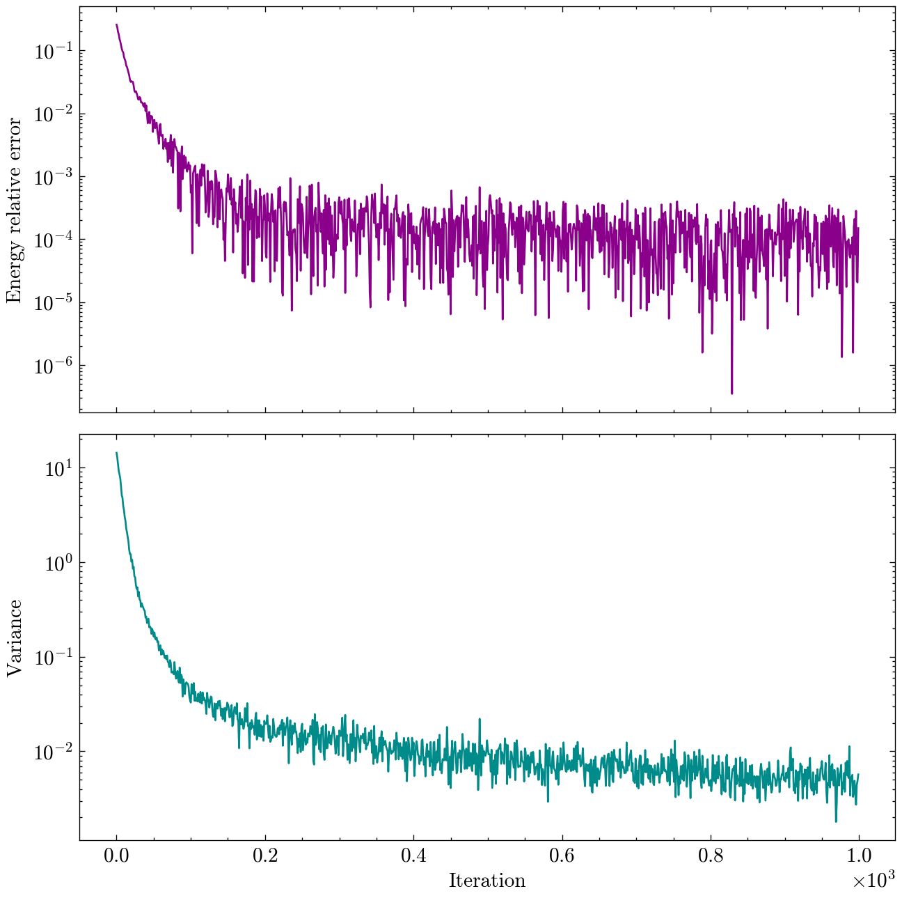
Finally, NetKet’s logging system allows us to easily track the optimization process and plot the results. In the following figure, we show the energy relative error and the energy variance as a function of iteration number.
As we can see, the energy relative error decreases by several orders of magnitude during the optimization, indicating that our MLP ansatz is successfully approximating the ground state of the TFIM at criticality. The energy variance also decreases, which is a sign that the state is becoming an eigenstate of the Hamiltonian.
Lastly, since since the exact ground state energy is known and the size of the system is still small, we can compute the exact (without sampling noise) energy of our final variational state and compare it to the exact ground state energy. We can also compute the exact infidelity between the final variational state and the exact ground state wavefunction.
Final energy: -15.3222 (relative error: 2.53e-05)
Final infidelity: 1.41e-04
Results are already pretty good, but with more iterations, a larger model, or more samples, we could further reduce the error and get even closer to the exact ground state energy.
Conclusions
Neural Quantum States (NQS) represent a genuine paradigm shift in quantum many-body physics. The core insight, pioneered by Carleo and Troyer, is that neural networks, as universal approximators with polynomial cost in the number of parameters, can learn the structure of a quantum state directly from the Hamiltonian, without the fixed architectural assumptions that constrain traditional ansätze. This flexibility, compatible with the use of rich informative priors, allows NQS to capture the complexity of quantum many-body systems in a way that was previously out of reach. By pairing the variational principle with automatic differentiation and stochastic gradient descent, NQS transform quantum state optimization into a scalable, hardware-accelerated procedure.
Beyond the practical advantages, NQS also offer a new lens for understanding the structure of the quantum states that nature actually chooses to realize. The fact that a neural network with polynomially many parameters can accurately represent a quantum state that nominally requires exponentially many amplitudes tells us something profound: physically relevant quantum states occupy a vanishingly small corner of Hilbert space, and that corner has learnable structure. In this sense, NQS could be as much a lens for understanding that compressibility as they are a computational tool for exploiting it.
That said, NQS remain far from a solved technology, with several deep challenges standing between current demonstrations and the large-scale problems they aspire to tackle. The sign problem (Westerhout et al. 2020; Troyer and Wiese 2005) is perhaps the most fundamental: capturing the non-trivial phase structure of frustrated magnets and fermionic systems is notoriously difficult for any naively parameterized ansatz, and NQS inherit this difficulty just as classical quantum Monte Carlo does. But this is not the only challenge. For example, stochastic reconfiguration, despite its geometric elegance, becomes a severe computational bottleneck as the number of samples and parameters grow. Additionally, the quality of MCMC sampling introduces its own silent hazards: poor mixing, high autocorrelation, and failures of ergodicity can quietly degrade results. More fundamentally, the field lacks a systematic theory bridging expressivity and learnability: the universal approximation theorem motivates the existence of a faithful representation, but says nothing about whether gradient-based optimization will find it, how many parameters it requires, or which architectures suit which classes of quantum states. Finally, unlike supervised learning, there is no held-out test set to catch failure: the only ground truth is exact diagonalization, available precisely for the small, tractable systems that NQS are meant to supersede.
Despite these challenges, the future of NQS is rich with possibility. On the one hand, the framework allows physicists to continuously leverage decades of rapid advancements in machine learning. For instance, symmetry preserving architectures with built-in lattice symmetries reduce parameter counts and improve generalization in precisely the way convolutional networks do for images (Lange et al. 2024), while autoregressive architectures, like transformers or recurrent networks, promise to eliminate MCMC sampling entirely (Sharir et al. 2020), removing autocorrelation and unlocking larger system sizes. On the other hand, the variational machinery extends naturally beyond ground states to excited states or real-time dynamics. Moreover, the NQS framework is not limited to spin systems: with appropriate modifications, it can be applied to fermionic systems, bosonic systems, and even continuous-variable systems, making it a versatile tool for a wide range of quantum many-body problems. In conclusion, the tools are open, the problems are deep, and the potential for discovery is immense.
Becca, Federico, and Sandro Sorella. 2017. Quantum MonteCarloApproaches for CorrelatedSystems. 1st ed. Cambridge University Press. https://doi.org/10.1017/9781316417041.
Carleo, Giuseppe, Kenny Choo, Damian Hofmann, et al. 2019. “NetKet: A Machine Learning Toolkit for Many-Body Quantum Systems.”SoftwareX 10 (July): 100311. https://doi.org/10.1016/j.softx.2019.100311.
Carleo, Giuseppe, and Matthias Troyer. 2017. “Solving the Quantum Many-Body Problem with Artificial Neural Networks.”Science 355 (6325): 602–6. https://doi.org/10.1126/science.aag2302.
Chen, Ao, and Markus Heyl. 2024. “Empowering Deep Neural Quantum States Through Efficient Optimization.”Nature Physics 20 (9): 1476–81. https://doi.org/10.1038/s41567-024-02566-1.
Hastings, W. K. 1970. “Monte Carlo Sampling Methods Using Markov Chains and Their Applications.”Biometrika 57 (1): 97–109. https://doi.org/10.1093/biomet/57.1.97.
Hornik, Kurt, Maxwell Stinchcombe, and Halbert White. 1989. “Multilayer Feedforward Networks Are Universal Approximators.”Neural Networks 2 (5): 359–66. https://doi.org/10.1016/0893-6080(89)90020-8.
Lange, Hannah, Anka Van de Walle, Atiye Abedinnia, and Annabelle Bohrdt. 2024. “From Architectures to Applications: A Review of Neural Quantum States.”Quantum Science and Technology 9 (4): 040501. https://doi.org/10.1088/2058-9565/ad7168.
Metropolis, Nicholas, Arianna W. Rosenbluth, Marshall N. Rosenbluth, Augusta H. Teller, and Edward Teller. 1953. “Equation of StateCalculations by FastComputingMachines.”The Journal of Chemical Physics 21 (6): 1087–92. https://doi.org/10.1063/1.1699114.
Rende, Riccardo, Luciano Loris Viteritti, Lorenzo Bardone, Federico Becca, and Sebastian Goldt. 2024. “A Simple Linear Algebra Identity to Optimize Large-Scale Neural Network Quantum States.”Communications Physics 7 (1): 260. https://doi.org/10.1038/s42005-024-01732-4.
Sharir, Or, Yoav Levine, Noam Wies, Giuseppe Carleo, and Amnon Shashua. 2020. “Deep AutoregressiveModels for the EfficientVariationalSimulation of Many-BodyQuantumSystems.”Physical Review Letters 124 (2): 020503. https://doi.org/10.1103/PhysRevLett.124.020503.
Vicentini, Filippo, Damian Hofmann, Attila Szabó, et al. 2022b. “NetKet 3: MachineLearningToolbox for Many-BodyQuantumSystems.”SciPost Physics Codebases, August, 7. https://doi.org/10.21468/SciPostPhysCodeb.7.
Westerhout, Tom, Nikita Astrakhantsev, Konstantin S. Tikhonov, Mikhail I. Katsnelson, and Andrey A. Bagrov. 2020. “Generalization Properties of Neural Network Approximations to Frustrated Magnet Ground States.”Nature Communications 11 (1): 1593. https://doi.org/10.1038/s41467-020-15402-w.
Wu, Dian, Riccardo Rossi, Filippo Vicentini, et al. 2024. “Variational Benchmarks for Quantum Many-Body Problems.”Science 386 (6719): 296–301. https://doi.org/10.1126/science.adg9774.
Footnotes
Two wave functions can yield the same measurement probabilities and represent different physical states.↩︎
This is done via tensor products. For example, \(\boldsymbol{\sigma}^{(2)}_z = \mathbb{1} \otimes \boldsymbol{\sigma}_z \otimes \mathbb{1} \otimes \cdots\).↩︎
This is the reason why we divide the expected value by \(\langle \psi_{\boldsymbol{\theta}} | \psi_{\boldsymbol{\theta}} \rangle\).↩︎
Its imaginary part is the Berry curvature, which measures the geometric phase/topology of the state manifold.↩︎