
Introduction
Grover’s algorithm is one of the most celebrated algorithms in quantum computing. It is a brilliant application of quantum principles to a fundamental computational problem: unstructured search. This is the problem of searching for an element in an unsorted list of \(N\) elements. An example of this type of problem would be searching for the name associated with a given number in a phone book, since entries are not ordered numerically but alphabetically. Classically, if you are handed an unsorted list of \(N\) items, where the elements are randomly distributed with equal probability, and you are told to find a specific one, you have no choice but to check them one by one. On average, you will need \(N/2\) checks; in the worst case, all \(N\). This is an algorithm with complexity \(\order{N}\). There is no clever trick or shortcut; you just have to grind through the possibilities. Grover’s algorithm tackles exactly this problem, but on a quantum computer, and it does so in just \(\order{\sqrt{N}}\) steps. That is a significant speedup. For a billion-entry database, that is a reduction from approximately \(5\times 10^{8}\) steps to \(3.2\times 10^4\). That is not just an improvement; it is a game changer.
However, this is not just about phone books. This type of search constitutes a fundamental problem in computation with multiple applications: finding the mean and median of a given set of values, finding the maximum or the minimum, finding more than one marked element, etc. In turn, this translates into specific applications in fields as important as finance, machine learning, chemistry, etc. In the following sections, Grover’s algorithm will be presented in detail, together with an example of code implementation using Qiskit. This tutorial is strongly based on the exposition made in (Nielsen and Chuang 2010) and the code from (various-authors 2023).
Problem Definition
First, we need to frame the search problem in a language a quantum computer can understand. Suppose we want to perform a search within an unsorted set, \(\mathcal{L}\), of \(N\) elements. To work with these elements, we will refer to their indices, from \(0\) to \(N-1\), instead of the elements themselves. For convenience, we will assume that \(N=2^n\) with \(n\in\N\), so that any index can be stored in \(n\) bits; that is, it can be encoded in the reading (measurement) of \(n\) qubits. Additionally, we will suppose that the search problem has exactly \(M\) solutions, with \(1\leq M\leq N\).
We will also assume that we have a quantum oracle \(O\), which can be imagined as a kind of black box capable of recognizing solutions to the search problem. Classicaly, the oracle for any search problem can be conveniently represented by a function \(f\) that receives as input an index \(x\in\{0, 1, \ldots, N-1\}\) and such that:
\[f(x) = \begin{dcases} 1 & \qif x \qq{is a solution}\\ 0 &\qq{otherwise}\end{dcases}.\]
In the quantum realm, this recognition can be manifested through an oracle qubit \(\ket{q}\). More specifically, the quantum oracle is a unitary operator \(O\) whose action on the computational basis is: \[\ket{x}\ket{q}\overset{O}{\mapsto}\ket{x}\ket{q\oplus f(x)},\] where \(\ket{x}\) is the quantum register of the index, \(\oplus\) denotes addition modulo 2, and \(\ket{q}\) is the oracle qubit, which inverts its value if and only if \(f(x)=1\), that is, if \(x\) is a solution to the search problem. In this way, it can be verified whether \(x\) is a solution to the problem simply by preparing the state \(\ket{x}\ket{0}\), applying the oracle \(O\), and checking whether the oracle qubit has changed from state \(\ket{0}\) to state \(\ket{1}\).
In reality, it is more useful to initialize the oracle qubit in the state \(\ket{-} = (\ket{0} - \ket{1})/\sqrt{2}\), since its action is then as follows: \[ \ket{x}\left(\frac{\ket{0}-\ket{1}}{\sqrt{2}}\right) \stackrel{O}{\mapsto}(-1)^{f(x)}\ket{x}\left(\frac{\ket{0}-\ket{1}}{\sqrt{2}}\right) . \] That is, if \(\ket{x}\) is a solution, then the global state is multiplied by \(-1\), meaning the amplitude of the global state becomes the opposite, but the state of the oracle qubit remains \(\ket{-}\). Since the state of the oracle qubit is not modified in any case, it can be omitted in what follows, remaining implicit and simplifying the exposition. Thus, we will simply write \[ \ket{x}\overset{O}{\mapsto}(-1)^{f(x)}\ket{x}. \] This phase flip is invisible if we measure immediately, but it becomes the foundation for quantum interference magic.
In conclusion, the oracle marks the solution to the search problem by changing the phase of the solution. This might feel like cheating. If the oracle can mark the solution, does it not already know the answer? Not at all. The oracle only needs to be able to verify a solution. It is a solution checker, not a finder. For our phonebook example, the oracle would be a circuit that takes a name, looks up its number, and compares it to the number we are searching for. We can build this checker without knowing in advance which name is the right one. The true challenge of Grover’s algorithm is to find the solutions to the search problem using as few calls to this oracle as possible. However, to be able to apply Grover’s algorithm, it will be necessary to efficiently construct a quantum circuit that implements the oracle for the specific problem being addressed. Grover’s algorithm only shows how to find solutions to a search problem once an oracle for that problem is available. Therefore, the details of the oracle, as well as the possibility of needing additional qubits to perform its operations, are not relevant to the description of Grover’s algorithm.
Grover’s Algorithm
Grover’s algorithm can be thought of as a clever process of amplitude amplification. We start with all possible answers having the same tiny amplitude, and then iteratively boost the amplitude of the correct answer while suppressing the others. Since the probability of measuring a quantum state is the square of its amplitude, Grover’s algorithm iteratively maximizes the probability of finding a solution to the problem when measuring the quantum register. Figure 1 schematically shows the quantum circuit that implements Grover’s algorithm.
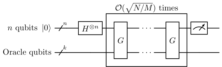
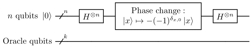
The algorithm employs a register of \(n\) qubits that is initialized in the state \(\ket{0}^{\otimes n}\). Subsequently, a Hadamard transformation \(H^{\otimes n}\) is applied to obtain the following superposition state: \[ % \ket{0}^{\otimes n}\stackrel{H^{\otimes n}}{\mapsto} \ket{\psi} = \frac{1}{\sqrt{N}} \sum_{x=0}^{N-1}\ket{x} . \] This superposition represents our quantum circuit considering all possibilities simultaneously. From this point, Grover’s algorithm consists of the repeated application of a subroutine known as the Grover iteration or Grover operator, \(G\). The circuit that implements this operator is shown in Figure 2 and Figure 3.
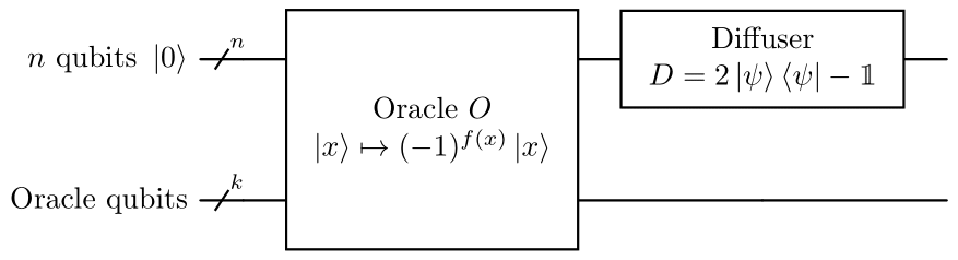
The Grover iteration consists of four steps:
- Apply the oracle \(O\).
- Apply a Hadamard transformation \(H^{\otimes n}\).
- Apply a conditional phase shift \(\ket{x} \mapsto-(-1)^{\delta_{x, 0}}\ket{x}\), with \(\delta_{i,j}\) the Kronecker delta.
- Apply a Hadamard transformation \(H^{\otimes n}\).
Each of the steps in the Grover iteration can, in principle, be implemented efficiently on a quantum computer. Steps 2 and 4, the Hadamard transformations, require \(n=\log(N)\) operations each. Step 3, the conditional phase shift, can be implemented with \(\order{n}\) gates. The cost of the oracle in step 1, however, depends on the specific problem being addressed.
Note that the conditional phase shift in step 3 can be implemented using the unitary operator \(2\ket{0}\bra{0} - \I\). Consequently, the action of steps 2, 3, and 4 is given by the so-called diffusion operator or diffuser: \[ D = H^{\otimes n}(2\ket{0}\bra{0}-\I) H^{\otimes n}=2\ket{\psi}\bra{\psi}-\I. \] When this operator is applied to a general state \(\sum_{k=0}^{N-1}\alpha_k\ket{k}\) the result is \[ \sum_{k=0}^{N-1}(-\alpha_k+2\langle\alpha\rangle)\ket{k}, \] where \(\ev{\alpha} = \sum_{k=0}^{N-1}\alpha_k/N\). In other words, the effect of this operator is an inversion of the amplitudes about their mean. Thus, the Grover operator can be written as an application of the oracle followed by an inversion about the mean of the amplitudes: \[G = (2\ket{\psi}\bra{\psi}-\I)O = D O.\] Since the oracle \(O\) inverts the amplitude of the solutions and leaves intact that of those states that are not solutions, if an inversion about the mean given by \(D\) is subsequently applied, the net effect is to amplify the amplitude of the solutions over the rest of the states. This is the effect of the Grover operator \(G\). Since the probability of measuring a state is the square of its amplitude, this operator must be applied repeatedly a sufficient number of times to maximize the probability of finding a solution to the problem when measuring the quantum register in the computational basis. This process is exemplified in Figure 4 for \(n=3\) (\(N=8\)).
Number of Iterations
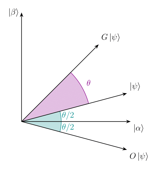
To be able to calculate the number of times it is necessary to apply the operator \(G\), it is convenient to visualize Grover’s algorithm geometrically. As will be seen below, the action of \(G\) can be seen as a rotation in the two-dimensional space spanned by the initial vector \(\ket{\psi}\) and the state formed by a uniform superposition of all solutions to the search problem. To see this, it is convenient to define the following states: \[ \begin{aligned} \ket{\beta} \equiv \frac{1}{\sqrt{M}} \sum_{\mathcal{S}}\ket{x}&\qq{with}\mathcal{S} = \{x\mid f(x)=1\},\\ \ket{\alpha} \equiv \frac{1}{\sqrt{N-M}} \sum_{\mathcal{L}-\mathcal{S}}\ket{x}&\qq{with}\mathcal{L}-\mathcal{S} = \{x\mid f(x)=0\}. \end{aligned} \] As can be seen, \(\ket{\beta}\) is a uniform superposition of all solutions to the search problem, while \(\ket{\alpha}\) is a uniform superposition of all states that are not solutions. With a little algebra, it can be seen that \[ \ket{\psi}=\sqrt{\frac{N-M}{N}}\ket{\alpha}+\sqrt{\frac{M}{N}}\ket{\beta}. \] For large \(N\) and small \(M\), this state is almost entirely in the \(\ket{\alpha}\) direction, with just a tiny component pointing toward our target, \(\ket{\beta}\). From the above expression, it is easy to see that the action of the oracle \(O\) on \(\ket{\psi}\) is a reflection about the vector \(\ket{\alpha}\) in the plane defined by \(\ket{\alpha}\) and \(\ket{\beta}\)1: \[O(a\ket{\alpha}+b\ket{\beta}) = a\ket{\alpha}-b\ket{\beta}.\] Similarly, the inversion about the mean operator, \(2\ket{\psi}\bra{\psi}-\I\), performs a reflection in the plane defined by \(\ket{\alpha}\) and \(\ket{\beta}\) about the vector \(\ket{\psi}\)2. And since the product of two reflections is a rotation, \(G\) can be interpreted as a rotation in the plane defined by \(\ket{\alpha}\) and \(\ket{\beta}\). Thus, \(G^k\ket{\psi}\) is contained in the plane defined by \(\ket{\alpha}\) and \(\ket{\beta}\) for all \(k\). To see the angle by which the state \(\ket{\psi}\) is rotated, \(\ket{\psi}\) can be rewritten as follows3: \[\ket{\psi} = \cos(\dfrac{\theta}{2})\ket{\alpha}+\sin(\dfrac{\theta}{2})\ket{\beta}\text{ with }\cos(\dfrac{\theta}{2}) = \sqrt{\dfrac{N-M}{N}}.\] Thus, we have \[G^k\ket{\psi} = \cos(\dfrac{2k+1}{2}\theta)\ket{\alpha}+\sin(\dfrac{2k+1}{2}\theta)\ket{\beta}.\] Therefore, the rotation angle is \(\theta\), that is, in the basis formed by \(\ket{\alpha}\) and \(\ket{\beta}\), we have \[G = \pmqty{\cos\theta & -\sin\theta\\ \sin\theta & \cos\theta}.\] The repeated application of \(G\) to \(\ket{\psi}\) brings the state of the quantum register closer to \(\ket{\beta}\) in steps of \(\theta\) radians.
Since the initial state of the system is \(\ket{\psi} = \sqrt{(N-M)/N}\ket{\alpha} + \sqrt{M/N}\ket{\beta}\), a rotation of \(\tilde{\theta} = \arccos\sqrt{M/N}\) radians results in \(\ket{\beta}\). Consequently, the number of times it is necessary to apply the operator \(G\) to maximize the probability of finding a solution is, therefore:
\[ R=\operatorname{CI}\pqty{\frac{\tilde{\theta}}{\theta}} = \operatorname{CI}\pqty{\frac{\arccos \sqrt{M / N}}{2\arccos\sqrt{(N-M)/N}}}, \]
where \(\operatorname{CI}\) denotes the closest integer. In Figure 6, \(R\) is represented as a function of \(M\) for multiple values of \(N\).

To better see what the behavior of \(R\) is with \(N\) and \(M\), it is convenient to try to simplify the above expression. For this, note that \(R \leq\lceil\pi / 2 \theta\rceil\)4, so that a lower bound of \(\theta\) provides an upper bound of \(R:\)
\[ \frac{\theta}{2} \geq \sin \frac{\theta}{2}=\sqrt{\frac{M}{N}}\Rightarrow R \leq\left\lceil\frac{\pi}{4} \sqrt{\frac{N}{M}}\right\rceil . \]
Here it can be clearly seen that \(R = \order{\sqrt{N/M}}\). This represents a quadratic improvement over the number of oracle queries in the classical case, \(\order{N/M}\). While it is beyond the scope of this work, it is possible to demonstrate that this improvement is optimal (Bennett et al. 1997; see Nielsen and Chuang 2010 for more details), that is, a quantum algorithm for this type of problem that is more efficient cannot be obtained.
Code Example with Qiskit
In this section, we will walk through a practical implementation of Grover’s algorithm using Qiskit, IBM’s open-source quantum computing framework. The following code cells will guide you step by step through the process of building and simulating Grover’s algorithm on a quantum circuit. Each cell is accompanied by an explanation to help you understand the purpose and logic behind the code, even if you have never used Qiskit before.
Dependencies
To begin, we import the necessary libraries from Qiskit and NumPy. Qiskit provides the tools to build and simulate quantum circuits, while NumPy is used for numerical operations. We also set up the AerSimulator, which allows us to run quantum circuits on a classical simulator, making it easy to test and visualize quantum algorithms without access to real quantum hardware.
import numpy as np
import qiskit
from qiskit import QuantumCircuit, transpile
from qiskit_aer import AerSimulator
from qiskit.visualization import plot_histogram

# Print versions for reproducibility
print(f"NumPy version: {np.__version__}")
print(f"Qiskit version: {qiskit.__version__}")

# Use Aer's AerSimulator
simulator = AerSimulator()
NumPy version: 2.3.5
Qiskit version: 2.3.0It is important to remember, from now on, that Qiskit orders its qubits in the reverse order to what is usual in the literature.
Initializer
Now we will define a function to initialize our quantum circuit. The goal is to create a uniform superposition over all possible states, which is the standard starting point for Grover’s algorithm. This is achieved by applying a Hadamard gate to each qubit in the circuit, ensuring that every possible state has equal probability amplitude:
def initializer(qc, qubits):
    # Apply a H-gate to 'qubits' in qc
    for q in qubits:
        qc.h(q)

    return qc
Oracle
The implementation of the oracle depends on the specific problem being addressed. As an example, we will create an oracle of little practical interest, but easy to understand. The following oracle will mark as solutions the states \(\ket{101}\) and \(\ket{110}\) for a register of 3 qubits:
oracle = QuantumCircuit(3)
# Multiply by -1 if |q2, q1, q0> = |101> or |110>
oracle.cz(0, 2) # Multiply by -1 if q0 = 1 and q2 = 1
oracle.cz(1, 2) # Multiply by -1 if q1 = 1 and q2 = 1
# We will return the oracle as a gate
oracle = oracle.to_gate()
oracle.name = "O"
In this way, \(n = 3\), \(N = 2^n = 8\), and \(M = 2\).
Diffuser
To create a general diffuser, recall that \[D = H^{\otimes n}(2\ket{0}^{\otimes n}\bra{0}^{\otimes n} -\I) H^{\otimes n}\] To implement the operator \((2\ket{0}^{\otimes n}\bra{0}^{\otimes n} -\I)\), we will use \(\operatorname{MCZ}\) (multi-controlled-Z) gates and \(X\) gates. On the one hand, \((2\ket{0}^{\otimes n}\bra{0}^{\otimes n} -\I)\) leaves unaffected the vector \(\ket{0}^{\otimes n}\) and inverts the phase of the rest of the basis vectors. On the other hand, an \(\operatorname{MCZ}\) gate inverts the phase of the state \(\ket{11\ldots 1}\) and leaves unaffected the rest of the basis vectors: \[ \operatorname{MCZ}= \pmqty{\dmat{1, 1, \ddots, -1}}. \] Therefore, we can implement \((2\ket{0}^{\otimes n}\bra{0}^{\otimes n} -\I)\) by transforming \(\ket{0}^{\otimes n}\) into \(\ket{1}^{\otimes n}\), applying an \(\operatorname{MCZ}\) gate, and then transforming back \(\ket{1}^{\otimes n}\) into \(\ket{0}^{\otimes n}\). The result will have a global \(-1\) factor. To map between \(\ket{0}^{\otimes n}\) and \(\ket{1}^{\otimes n}\), we can use \(X\) gates: \[ \begin{aligned} X^{\otimes n}\ket{0}^{\otimes n} &= \ket{1}^{\otimes n}, \\ X^{\otimes n}\ket{1}^{\otimes n} &= \ket{0}^{\otimes n}. \end{aligned} \] Thus, \[2\ket{0}^{\otimes n}\bra{0}^{\otimes n} -\I = -X^{\otimes n}\operatorname{MCZ} X^{\otimes n}.\] Therefore, the diffusion operator \(D\) can be constructed as \[ D=-H^{\otimes n} X^{\otimes n}\operatorname{MCZ} X^{\otimes n} H^{\otimes n}. \] Moreover, since a global phase change is irrelevant, the factor \(-1\) in the expression for \(D\) can be ignored.
On many real quantum computers, the Multi-Controlled Z gate is not a native operation. It must be decomposed into simpler, more fundamental gates. A common way to implement an \(\operatorname{MCZ}\) is using a Multi-Controlled X5 (\(\operatorname{MCX}\)) gate, flanked by Hadamards on the target qubit. Therefore, the implementation of a diffuser in Qiskit is as follows:
def diffuser(nqubits):
    qc = QuantumCircuit(nqubits)
    # Apply transformation |psi> -> |00...0> (H-gates)
    for qubit in range(nqubits):
        qc.h(qubit)
    # Apply transformation |00...0> -> |11...1> (X-gates)
    for qubit in range(nqubits):
        qc.x(qubit)
    # Do multi-controlled-Z gate
    qc.h(nqubits-1)
    qc.mcx(list(range(nqubits-1)), nqubits-1)  # multi-controlled-toffoli
    qc.h(nqubits-1)
    # Apply transformation |11...1> -> |00...0>
    for qubit in range(nqubits):
        qc.x(qubit)
    # Apply transformation |00...0> -> |psi>
    for qubit in range(nqubits):
        qc.h(qubit)
    # We will return the diffuser as a gate
    D = qc.to_gate()
    D.name = "D"

    return D
Grover Operator
Now that we have both the oracle and the diffuser, we combine them into the Grover operator. This operator encapsulates one full iteration of Grover’s algorithm: first applying the oracle to mark the solutions, then the diffuser to amplify their amplitudes. By packaging these steps together, we can easily repeat the Grover iteration as many times as needed.
def grover_operator(nqubits, oracle):
    # Create quantum circuit
    qc = QuantumCircuit(nqubits)
    # Append oracle
    qc.append(oracle, range(n))
    # Append diffuser
    qc.append(diffuser(n), range(n))
    # We will return the grover operator as a gate
    G = qc.to_gate()
    G.name = "G"

    return G
Complete Circuit
With all the building blocks in place, we define a function to assemble the complete Grover circuit. This function initializes the quantum register, determines the optimal number of Grover iterations based on the problem size and number of solutions, and applies the Grover operator the appropriate number of times. Finally, it measures the qubits, allowing us to extract the result of the quantum search.
def grover_circuit(n, M, oracle):
    N = 2**n
    # Create quantum circuit
    qc = QuantumCircuit(n, n)
    # Initialize the state to a superposition
    qc = initializer(qc, range(n))
    # Define the number of iterations
    iterations = round(np.arccos(M/N)/(2*np.arccos(np.sqrt((N-M)/N))))
    # Apply Grover's iterations
    for _ in range(iterations):
        qc.append(grover_operator(n, oracle), range(n))

    # Measure the qubits
    qc.measure(range(n), range(n))

    return qc
Example of Use
Now we create an instance of the Grover circuit for our example problem, specifying the number of qubits and solutions. We then visualize the resulting quantum circuit, which provides insight into the structure and sequence of operations that implement Grover’s algorithm.
n, M = 3, 2
qc = grover_circuit(n, M, oracle)
# Print the circuit
# print("Quantum Circuit:", qc)
# Plot the circuit
qc.draw(output='mpl', style='clifford')
Finally, we simulate the execution of the Grover circuit using the AerSimulator. By running the circuit multiple times, we obtain a histogram of measurement outcomes.
# Simulate the circuit
compiled_circuit = transpile(qc, simulator)
job = simulator.run(compiled_circuit, shots=10000)
result = job.result()
# Get and print the result
counts = result.get_counts(compiled_circuit)
# print("Measurement results:", counts)
plot_histogram(counts, bar_labels=False)
The two bars correspond to the states \(\ket{101}\) and \(\ket{110}\), which are the states marked as solutions by the oracle. Both states appear with nearly equal frequency, while all other states have zero counts. Therefore, the simulation validates the correct implementation of Grover’s algorithm and its ability to efficiently identify the marked solutions in an unstructured search problem.
Challenges and Limitations
Despite its theoretical beauty, Grover’s algorithm faces practical hurdles:
- Quantum Error Correction: Grover’s algorithm requires maintaining quantum coherence over many qubits and multiple iterations. Current quantum computers struggle with the error rates required for large-scale Grover implementations.
- Oracle Overhead: For many problems, the quantum oracle requires more resources than the classical problem itself. The art lies in finding problems where the oracle is naturally efficient.
- Classical Competition: As quantum hardware advances, so do classical algorithms and hardware. In some cases, improvements in classical search or optimization methods can reduce or even eliminate the practical advantage of Grover’s algorithm.
- Data Input and Output: Loading classical data into a quantum state (quantum data encoding) and extracting useful information from quantum measurements can introduce significant overhead, often offsetting the theoretical speedup.
- Limited Speedup: Grover’s algorithm provides a quadratic, not exponential, speedup. For very large search spaces, this is significant, but it does not make intractable problems suddenly easy.
Conclusion
Grover’s algorithm is a landmark result in quantum computing, elegantly demonstrating how quantum interference can be harnessed to solve unstructured search problems more efficiently than any classical approach. Rather than checking multiple items in parallel in the classical sense, Grover’s algorithm uses amplitude amplification: the probability amplitudes of incorrect answers interfere destructively, while the correct answer is constructively amplified. It is not about checking things faster; it is about making the wrong answers cancel each other out, leaving only the right one standing tall. It is a fundamentally different and powerful way to compute.
Grover’s algorithm represents something profound about quantum computing. Unlike Shor’s algorithm, which exploits the specific mathematical structure of factoring, Grover’s algorithm works for completely unstructured problems. It shows that quantum mechanics provides a genuine, if limited, advantage for a very general class of computational problems. As a consequence, it represents a new way of thinking about search and optimization whose applications extend far beyond database search. Additionally, Grover’s algorithm is optimal—no quantum algorithm can solve the unstructured search problem in fewer than \(O(\sqrt{N/M})\) queries (Bennett et al. 1997). While this is a quadratic, not exponential, speedup, it is nonetheless significant for large search spaces. Therefore, as quantum hardware matures, Grover’s algorithm and its variants will likely play important roles in practical quantum applications.
This algorithm reshapes our understanding of what it means to search, turning a brute-force task into an elegant geometric rotation. It is a cornerstone of the quantum algorithmic toolkit and a powerful reminder that computation, at its deepest level, is physical. Ultimately, Grover’s algorithm reminds us that some of the most profound advances in computation come not from exploiting special structure, but from finding fundamentally new ways to harness the laws of nature.
References
Bennett, Charles H., Ethan Bernstein, Gilles Brassard, and Umesh Vazirani. 1997. “Strengths and Weaknesses of Quantum Computing.” SIAM Journal on Computing 26 (5): 1510–23. https://doi.org/10.1137/S0097539796300933.
Galindo, Alberto, and Miguel A. Martin-Delgado. 2000. A Family of Grover’s Quantum Searching Algorithms. https://doi.org/10.48550/ARXIV.QUANT-PH/0009086.
Galindo, A., and M. A. Martín-Delgado. 2002. “Information and Computation: Classical and Quantum Aspects.” Reviews of Modern Physics 74 (2): 347–423. https://doi.org/10.1103/RevModPhys.74.347.
Grover, Lov K. 1996. A Fast Quantum Mechanical Algorithm for Database Search. https://doi.org/10.48550/ARXIV.QUANT-PH/9605043.
Nielsen, Michael A., and Isaac L. Chuang. 2010. Quantum Computation and Quantum Information. 10th anniversary ed. Cambridge University Press.
Footnotes
Remember that \(O\) multiplies by \(-1\) the amplitude of the solution states.↩︎
The term \(2\ket{\psi}\bra{\psi}\) projects any vector along \(\ket{\psi}\) and multiplies it by two. The term \(-\I\) subtracts the original vector from this quantity, so the component along \(\ket{\psi}\) remains the same but the orthogonal component changes its sign. As a result, the vector is reflected about \(\ket{\psi}\).↩︎
Since \(\ket{\psi}\) is normalized.↩︎
Since \(\sqrt{M/N} \geq 0\), necessarily \(0 \leq \arccos\sqrt{M/N} \leq \pi/2\).↩︎
Also known as Multi-Controlled NOT or Multi-Controlled Toffoli.↩︎