Graph Neural Networks (GNNs) extend deep learning to graph-structured data by respecting permutation symmetries. This post explores the mathematical foundations, different GNN flavors (convolutional, attentional, and message-passing), and provides hands-on PyTorch Geometric implementations.
Geometric DL
PyTorch
Published
September 8, 2025
Introduction
In the world of deep learning, we have grown accustomed to architectures that thrive on order and structure. Most of us first encounter neural networks in their simplest form: as Multilayer Perceptrons (MLPs), mapping a fixed-size vector input in \(\R^D\) to another vector or scalar output. Later, we learn how convolutional layers exploit the rigid grid structure of images, leveraging translational symmetry, or how recurrent networks exploit the sequential structure of text or time series.
But what happens when our data does not fit into these neat, ordered boxes? What if the structure is the data itself? Think of molecules (atoms linked by chemical bonds), social networks (users linked by friendships), or transportation systems (stations linked by routes). These structures are not naturally described by vectors, grids, or sequences, but by graphs. A graph is simply a collection of entities (nodes) and the connections (edges) between them, and it is one of the most natural and flexible ways to represent complex data. In fact, many other data structures, such as sets and grids, can also be represented as graphs.
One important aspect of this domain is that the order in which you list the nodes is completely arbitrary—the underlying network remains the same. However, an MLP trained on one ordering would produce a completely different result for another, even if the graph is identical. This presents a fundamental challenge: how do we design a neural network that is inherently indifferent to the order of its inputs? This property is called permutation invariance, and building it into the structure of our models is the core idea behind Graph Neural Networks (GNNs).
GNNs represent one of the most significant advances in deep learning, extending our ability to learn from data that lives on graphs rather than grids or sequences. They are part of the broader framework of Geometric Deep Learning (Bronstein et al. 2017), which seeks unifying principles across architectures by respecting the symmetries of their input domains. To learn more about this field, check out (Bronstein et al. 2021)1, which has been the main reference for this post.
Formalizing the Challenge
To build a principled model to learn from graph-structured data, we first need to introduce the mathematical formalism to describe this type of data and its inherent symmetries.
Graphs
A graph is defined as a pair \(G = (\mathcal{V}, \mathcal{E})\), where \(\mathcal{V} = \{1, \dots, N\}\) is a set of \(N\equiv |\mathcal{V}|\) nodes (or vertices) and \(\mathcal{E} \subseteq \mathcal{V} \times \mathcal{V}\) is a set of edges (or links) connecting pairs of those nodes. Think of nodes as entities and edges as relationships between them:
In a social network: nodes are users, edges are friendships.
In a molecule: nodes are atoms, edges are chemical bonds.
In a citation network: nodes are papers, edges are citations.
The graph’s connectivity is also represented by an adjacency matrix \(\vb{A} \in \{0, 1\}^{N \times N}\), where \(A_{u, v}=1\) if and only if \((u,v)\in \mathcal{E}\). If \(A_{u, v} = A_{v, u}\;\forall u,v \in \mathcal{V}\), the graph is said to be undirected; otherwise, it is directed. The number of connections of each node is the so called the degree of the node:
Each node \(v \in \mathcal{V}\) may have an associated feature vector \(\vb{x}_v \in \R^D\)—for example, a user’s profile information in a social network or an atom’s chemical properties in a molecule. We can stack these \(D\)-dimensional feature vectors into a node feature matrix \(\vb{X} = (\vb{x}_1, \ldots, \vb{x}_N)^\top \in \R^{N \times D}\). Additionally, edges \((u,v) \in \mathcal{E}\) may have features \(\vb{e}_{u, v}\in \R^M\). Sometimes, these edge features are scalars representing weights, which can be incorporated into the adjacency matrix \(\vb{A}\), allowing for weighted graphs. In this case, the entries of \(\vb{A}\) are real-valued, representing the strength or capacity of the connections between nodes. To simplify the notation, we will omit the edge features in the following sections, but they can be easily incorporated into the models we will discuss without changing the underlying principles.
Permutation Symmetry
The critical insight about graphs is that the specific ordering of the \(N\) nodes—for example, when building \(\vb{X}\) and \(\vb{A}\)—is an artifact of our representation, not a property of the graph itself. Unlike the pixels of an image or the elements of a time series, the nodes of a graph do not have a natural ordering. Relabeling the nodes of a graph does not change the graph itself. If we shuffle, or permute, the nodes, we get a different feature matrix \(\vb{X}'\) and adjacency matrix \(\vb{A}'\), but they represent the exact same graph. This shuffling can be represented by a \(N \times N\) permutation matrix \(\vb*{\Pi}\) (exactly one 1 in each row and column, zeros elsewhere). Applying this permutation to our graph data transforms the feature matrix by reordering its rows (\(\vb{X}' = \vb*{\Pi}\vb{X}\)) and the adjacency matrix by reordering both its rows and columns (\(\vb{A}' = \vb*{\Pi}\vb{A}\vb*{\Pi}^\top\)).
This creates a fundamental challenge. Depending on the task, our neural network must satisfy one of two conditions:
Permutation Invariance (Graph-level tasks): If our goal is to predict a single property for the entire graph (e.g., a molecule’s toxicity), the output must be identical regardless of node ordering. A function \(f\) is permutation invariant if, for any permutation matrix \(\vb*{\Pi}\), it holds that: \[f(\vb*{\Pi}\vb{X}, \vb*{\Pi}\vb{A}\vb*{\Pi}^\top) = f(\vb{X}, \vb{A}).\]
Permutation Equivariance (Node-level tasks): If we are predicting a property for each node (e.g., classifying users in a social network), then permuting the input nodes should result in the same permutation of the output node properties. A function \(\vb{F}\) that outputs a new \(N \times D'\) matrix of node features is permutation equivariant if: \[\vb{F}(\vb*{\Pi}\vb{X}, \vb*{\Pi}\vb{A}\vb*{\Pi}^\top) = \vb*{\Pi}\vb{F}(\vb{X}, \vb{A}).\]
Any architecture we design for graphs must satisfy these conditions by its very structure. This is not just an academic exercise; it is a powerful inductive bias that dramatically reduces the search space of functions our model has to learn, leading to better generalization and data efficiency.
Graph Neural Networks
So, how do we build a neural network that respects these symmetries? Graph Neural Networks are the answer. The key idea behind GNNs is to iteratively update node features, also called node embeddings (representations), by aggregating information from their local neighborhoods. This process is often referred to as message passing or graph convolution. A GNN layer is a function of the form
where \[
\mathcal{N}_u = \{v : (u,v) \in \mathcal{E} \text{ or } (v,u) \in \mathcal{E}\}
\] is the neighborhood of a node \(u\), the set of all nodes connected to it by an edge2, and
\[
\mathbf{X}_{\mathcal{N}_u} = \{\{\mathbf{x}_v : v \in \mathcal{N}_u\}\}
\]
is the multiset (set with possible repetitions3) of feature vectors of its neighbors. The function \(\varphi\) takes as input the feature vector of the node itself, \(\vb{x}_u\), and the multiset of feature vectors of its neighbors, \(\mathbf{X}_{\mathcal{N}_u}\), and produces a new feature vector for that node.
It is important to note that \(\vb{F}\) is constructed by applying a shared function \(\varphi\) to each node locally, so \(\vb{F}\) is permutation equivariant if \(\varphi\) is permutation invariant, that is, if the output of \(\varphi\) does not depend on the ordering of the nodes in \(\mathcal{N}_u\). The way GNNs achieve this is by using a permutation-invariant aggregation function, \(\bigoplus\) (like sum, mean, or max), to combine the information from the neighbors into a single vector that does not depend on their order: \[\vb{m}_{\mathcal{N}_u} = \bigoplus_{v \in \mathcal{N}_u}\psi(\vb{x}_u, \vb{x}_v).\]
The function \(\psi\), typically a learnable function, is called the message function, and the vectors
\[\vb{m}_{v,u} = \psi(\vb{x}_u, \vb{x}_v)\]
are called messages4 from neighbor \(v\) to the central node \(u\). On the other hand, the function \(\varphi\), usually a learnable function too, is called the update function, since it updates the node’s features based on the aggregated information from its neighbors, \(\vb{m}_{\mathcal{N}_u}\), and its own features, \(\vb{x}_u\): \[
\vb{h}_u = \varphi(\vb{x}_u, \vb{m}_{\mathcal{N}_u}),
\] where \(\vb{h}_u\) is the new feature vector for node \(u\). Stacking these layers allows information to propagate across the graph; after \(k\) layers, the representation of a node is influenced by its \(k\)-hop neighborhood.
The Three Flavors
Most GNN architectures in the literature can be categorized into three “flavors”, distinguished by the structure of the message function \(\psi\): convolutional, attentional, and message-passing. Each flavor includes the previous one as a special case and offers a different balance of simplicity, expressiveness, and computational cost. All three flavors share the same overall structure, but differ in how they compute the messages from neighbors.
Convolutional GNNs
This is the simplest flavour, where the message, \(\vb{m}_{v,u}\), from a neighbor is simply its own features, \(\vb{x}_v\), transformed by some function, \(\phi\), and weighted by a predefined constant coefficient, \(c_{v, u}\):
The coefficients \(c_{v, u}\) are typically derived from the graph structure itself. For example, they could be based on the node degrees from the adjacency matrix. This operation acts like a diffusion or filtering process on the graph, which is why it is analogous to convolution on a grid.
Attentional GNNs
Instead of using fixed weights, attentional GNNs allow the model to learn the importance of each neighbor dynamically, based on node features5. The message from neighbor \(v\) is weighted by an attention coefficient \(\alpha_{v, u}\), computed by a function \(a: \R^D \times \R^D \rightarrow \R\):
The attention mechanism \(a\) allows the model to assign higher weights to more relevant neighbors, making the information aggregation more flexible and powerful. This is the same principle that powers the famous Transformer architecture, which can be viewed as an attentional GNN on a fully-connected graph of words (Joshi 2025).
Note that convolutional GNNs are a special case of attentional GNNs where the attention coefficients are fixed and do not depend on the node features: \(a(\vb{x}_u, \vb{x}_v) = c_{v, u}\).
Message-Passing GNNs
This is the most general and expressive flavour. Here, the message from neighbor \(v\) to \(u\) can be any learnable function of both nodes’ features6:
This allows the model to capture complex interactions between nodes. In fact, both convolutional and attentional GNNs are special cases of message-passing GNNs with specific forms of the message function \(\psi\), since we can always write \(\psi(\vb{x}_u, \vb{x}_v) = a(\vb{x}_u, \vb{x}_v)\phi(\vb{x}_v)\). However, this does not imply that message-passing GNNs are always the most useful variant. In fact, they are typically harder to train and require more computational resources.
The Geometric Deep Learning Blueprint
The Geometric Deep Learning (GDL) Blueprint (Bronstein et al. 2017, 2021) provides a unified framework for understanding architectures like CNNs, GNNs, and Transformers. It sees them as networks that respect the geometry and symmetries of their input domains. According to the GDL blueprint, for a deep learning architecture to effectively process elements of a domain \(\Omega\) under a symmetry described by a certain group \(\mathfrak{G}\), it must be properly constructed using the following key building blocks:
Linear \(\mathfrak{G}\)-equivariant layer: A layer satisfying \(F(g\cdot x) = g\cdot F(x),\;\forall g\in\mathfrak{G}\). If you transform the input, the output transforms in the same way.
Nonlinearity: An activation function applied element-wise.
Local pooling (coarsening): An operator that reduces the resolution of the domain, such that the new domain is a compact version of the original.
\(\mathfrak{G}\)-invariant layer (global pooling): A layer satisfying \(F(g\cdot x) = F(x),\;\forall g\in\mathfrak{G}\). They produce an output that is insensitive to the domain’s symmetries.
For example, classical convolutional layers are equivariant layers that respect translational symmetry for grid-like data, such as images. In the case of GNNs, the input domain consists of graphs and the corresponding symmetry group is the permutation group, \(S_n\). Let us examine the architecture of GNNs through this lens:
The message-passing operation \(\psi\) can be seen as a permutation-equivariant layer, since it is applied pairwise to neighboring nodes.
The aggregation function \(\bigoplus\) is a permutation-invariant operation that combines messages from neighboring nodes, and the definition of neighboring nodes \(\mathcal{N}_u\) is also invariant to permutations.
The update function \(\varphi\) is a permutation-equivariant layer, as it is a node-wise operation on the node features and its aggregated messages, which is an invariant quantity, as we have just seen.
As a result, the entire layer is a permutation-equivariant function.
This unified perspective helps us understand why these architectures work so well. They are not just collections of layers that perform well empirically; they are principled constructions that correctly embed the fundamental symmetries of the data they are designed for. As we have already noted, this is a powerful inductive bias that dramatically reduces the search space of functions our model has to learn, leading to better generalization and data efficiency.
Applications
The ability to learn from graph-structured data unlocks a vast array of problems and applications across science and industry. First, these tasks can be classified into two categories depending on the experimental setting:
Transductive learning: The model is trained and evaluated on the same graph. The model has access to the entire graph structure (all nodes and edges) during training, but labels are only available for a subset of nodes. The model must predict labels for the unlabeled nodes in the same graph; no new nodes or graphs appear at test time. This is a semi-supervised learning problem.
Inductive learning: The model is trained on one graph and evaluated on a different unseen graph. The model must generalize to completely unseen nodes or even entirely new graphs that were not present during training.
Second, tasks can be categorized by the level at which predictions are made:
Node-level tasks: For these problems, a property for each node is predicted. This requires a stack of equivariant GNN layers. For example, in social networks, we might want to make predictions about users from a social network or classify each paper’s topic in a citation network.
Edge-level tasks: Also known as link prediction, this involves predicting whether a connection exists between two nodes, classifying the type of connection, or inferring a continuous property of it (strength, flow, rating, etc.). This is useful, for instance, in recommender systems, where GNNs predict user-item interactions by modeling users and items as nodes in a graph.
Graph-level tasks: For these tasks, we need to predict a single property for the entire graph. This requires an invariant model, typically achieved by applying a global pooling (readout) layer and a MLP after the final GNN layer. As an example, GNNs can predict molecular properties such as solubility or toxicity from a molecule’s graph.
These learning problems can also belong to different training regimes (supervised, unsupervised, semi-supervised, self-supervised), and their applications are numerous and span diverse fields: materials science, molecular modeling, social network analysis, recommendation systems, traffic forecasting and logistics, fraud detection, and more.
Code Example with PyTorch Geometric
In this section, we will explore the implementation of GNNs using the PyTorch Geometric library. For each flavor of GNN, we will provide a simple code example of a particular architecture. We will make use of the QM9 dataset for our examples, which is a widely used benchmark dataset for molecular property prediction.
Dependencies
Apart from NumPy and some visualization libraries, such as Matplotlib and Py3Dmol, the main dependencies for our GNN implementations are PyTorch and PyTorch Geometric. PyTorch Geometric is a library built on top of PyTorch that provides tools for working with graph-structured data. After we import the necessary libraries, we will set the random seed for reproducibility and the device for computation.
For this tutorial, our playground is the QM9 dataset, and our game is to predict the molecular dipole moment. QM9 is made up of 130,831 small molecules, each represented as a graph where atoms are nodes and chemical bonds are edges. The molecules in QM9 are composed of up to nine heavy atoms—Carbon (C), Nitrogen (N), Oxygen (O), and Fluorine (F)—along with Hydrogen (H) atoms. But this dataset is more than just a list of molecules. For each one, a set of 19 quantum mechanical properties has been calculated and included. These are not experimental measurements, but the result of sophisticated computer simulations using a method called Density Functional Theory (DFT). For all of this, QM9 provides a standardized benchmark for developing and testing GNNs.
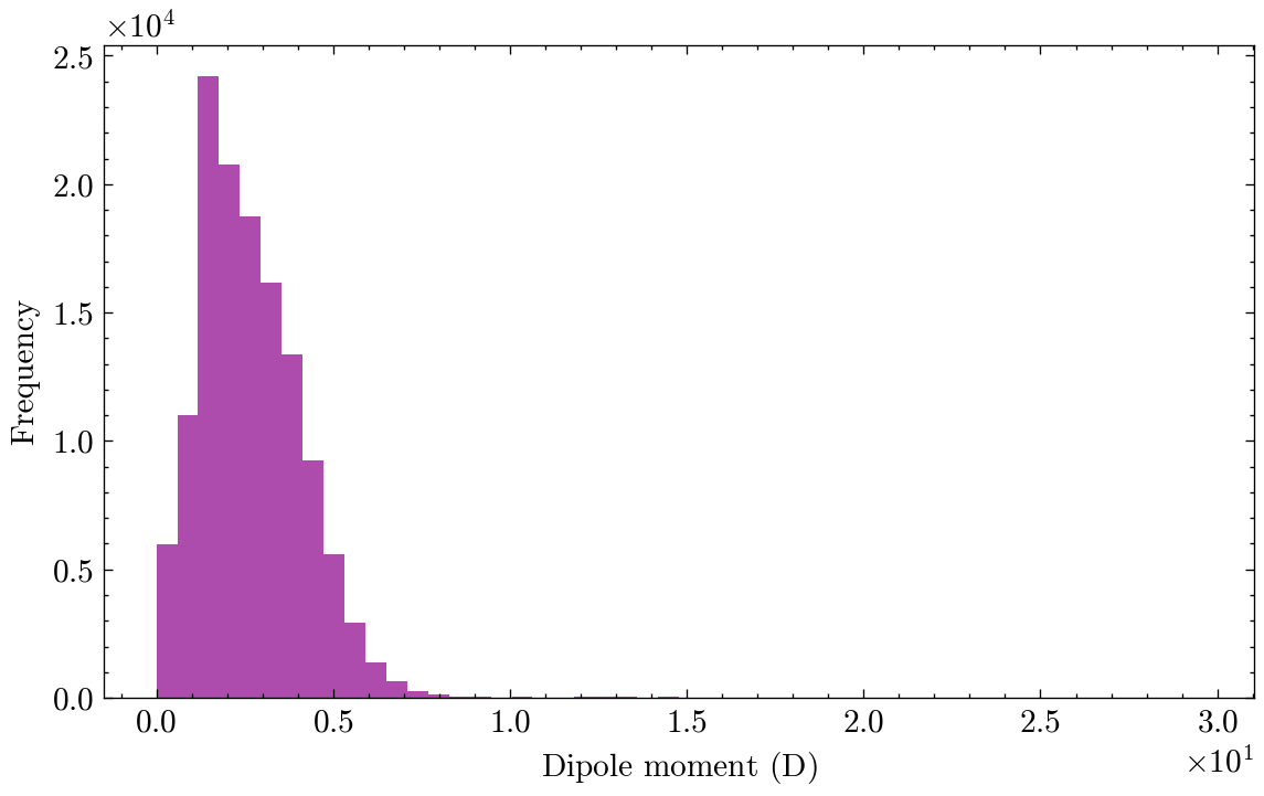
Among the 19 properties in QM9, we will focus on one in particular: the dipole moment, \(\mu\). In simple terms, a molecule’s dipole moment is a measure of its overall polarity. It arises from the unequal sharing of electrons between atoms in a chemical bond. Some atoms, such as oxygen and fluorine, are more electronegative, meaning they pull electrons more strongly toward themselves. When a bond forms between atoms with different electronegativities, the electrons spend more time around the more electronegative atom. This creates a slight negative charge on that atom and a slight positive charge on the less electronegative one. This separation of charge is called a bond dipole.
A dipole moment is a vector quantity, meaning it has both a magnitude (how large the charge separation is) and a direction (pointing from the positive to the negative charge). The overall dipole moment of a molecule is the vector sum of all its individual bond dipoles. This is where the 3D geometry of a molecule becomes critically important.
In a molecule such as carbon dioxide (CO₂), the two oxygen atoms are pulling electrons away from the central carbon atom. However, because the molecule is linear and symmetrical, these two bond dipoles are equal in magnitude and opposite in direction. They perfectly cancel each other out, and the molecule as a whole has a dipole moment of zero, making it nonpolar.
In contrast, a water molecule (H₂O) has a bent shape. The two hydrogen atoms are on one side of the oxygen atom. The bond dipoles from the O-H bonds do not cancel out; instead, they add up to give the molecule a net dipole moment, making it polar.
The standard unit for the dipole moment is the Debye (D), and this is the unit used in the QM9 dataset.
Predicting the dipole moment is a fantastic challenge for a GNN. It is not enough to know which atoms are in a molecule; the model must also understand their spatial arrangement and the electronic interactions. This makes it a perfect task to showcase the power of graph-based learning.
To load the QM9 dataset, we will use the QM9 class from PyTorch Geometric. We will also apply some transformations to the data. First, we will select only the target property we want to predict (dipole moment) using a custom transform. Then, we will compute the pairwise distances between atoms and add them as edge features using the Distance transform.
num_node_features = dataset.num_node_featuresnum_edge_features = dataset.num_edge_featuresprint("Dataset properties:")print(f" Number of molecules: {len(dataset)}")print(f" Number of features per atom: {num_node_features}")print(f" Number of edge features: {num_edge_features}")molecule = dataset[0]print("Sample molecule:")print(f" Number of atoms: {molecule.x.shape[0]}")print(f" Nodes features shape: {molecule.x.shape}")print(f" Edges shape: {molecule.edge_index.shape}")print(f" Edges features shape: {molecule.edge_attr.shape}")print(f" Target shape: {molecule.y.shape}")
Dataset properties:
  Number of molecules: 130831
  Number of features per atom: 11
  Number of edge features: 5
Sample molecule:
  Number of atoms: 5
  Nodes features shape: torch.Size([5, 11])
  Edges shape: torch.Size([2, 8])
  Edges features shape: torch.Size([8, 5])
  Target shape: torch.Size([1, 1])
The number of atoms varies from molecule to molecule, but the number of features per atom is always 11:
1st-5th features: a one-hot encoding of the atom type (H, C, N, O, F).
6th feature: the atomic number (number of protons).
7th feature: indicates whether the atom is aromatic (binary).
8th-10th features: a one-hot encoding of the electron orbital hybridization (sp, sp2, sp3).
11th feature: the number of hydrogens attached to the atom.
The edges are represented in COO format by the edge_index tensor, which has shape [2, num_edges], where each column represents a directed edge [source_node, target_node]. Each edge has five features:
1st-4th features: a one-hot encoding of the bond type (single, double, triple, aromatic),
5th feature: the Euclidean distance between the two atoms connected by the bond.
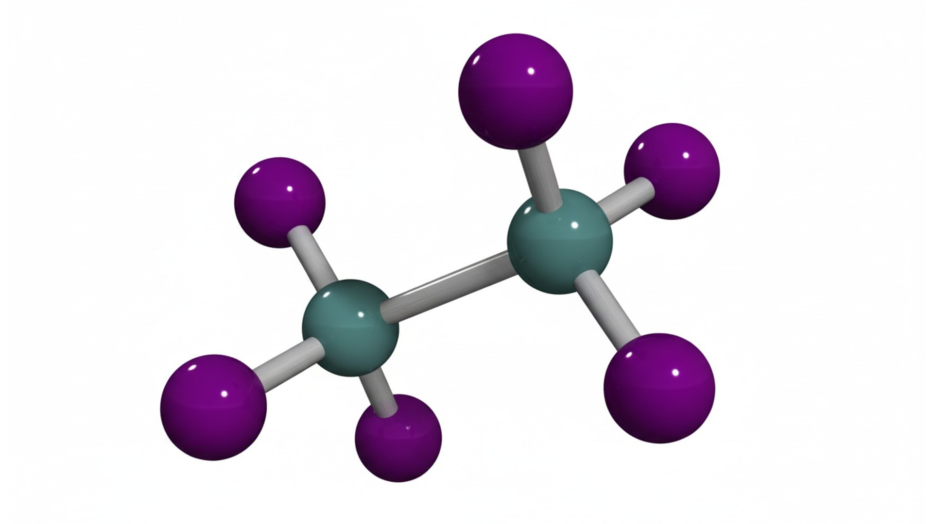
We can also visualize some molecules from the dataset using Py3Dmol, which allows us to interact with the 3D structures (rotate, zoom, etc.). Give it a try!
Code
ATOM_LABELS = {1: "H", 6: "C", 7: "N", 8: "O", 9: "F"}ATOM_SIZES = {k: 30for k in ATOM_LABELS}palette = plt.rcParams['axes.prop_cycle'].by_key()['color']ATOM_COLORS = {k: palette[i] for i, k inenumerate(ATOM_LABELS)}# Bond type configurationBOND_TYPES = {0: "single", # First position in one-hot1: "double", # Second position in one-hot2: "triple", # Third position in one-hot3: "aromatic"# Fourth position in one-hot}# Bond visual propertiesBOND_STYLES = {"single": {"radius": 0.08,"color": "#C0C0C0", # Light gray"opacity": 0.8 },"aromatic": {"radius": 0.10,"color": "#808080", # Medium gray"opacity": 0.7 },"double": {"radius": 0.12,"color": "#404040", # Dark gray"opacity": 0.9 },"triple": {"radius": 0.15,"color": "#202020", # Very dark gray"opacity": 1.0 }}def decode_bond_type(edge_attr_vector):""" Decode the one-hot vector to determine bond type Args: edge_attr_vector: First 4 elements of edge attribute (one-hot encoded) Returns: Bond type string """# Find the position of the 1 in the one-hot vector bond_type_idx = np.argmax(edge_attr_vector[:4])return BOND_TYPES[bond_type_idx]def visualize_molecule_py3dmol(molecules, ncols=2, initial_zoom=1.5):"""Use py3Dmol for molecular visualization in a grid layout with independent controls"""import math nrows = math.ceil(len(molecules) / ncols)# Create a grid viewer with linked=False for independent interaction viewer = py3Dmol.view( width=300* ncols, height=300* nrows, viewergrid=(nrows, ncols), linked=False )for idx, molecule inenumerate(molecules): row = idx // ncols col = idx % ncols# Get data pos = molecule.pos.numpy() atomic_numbers = molecule.z.numpy() edge_index = molecule.edge_index.numpy() edge_attr = molecule.edge_attr.numpy()# Add atoms as spheres to specific grid positionfor position, atomic_num inzip(pos, atomic_numbers): viewer.addSphere({'center': {'x': float(position[0]),'y': float(position[1]),'z': float(position[2]) },'radius': ATOM_SIZES[int(atomic_num)] /100,'color': ATOM_COLORS[int(atomic_num)] }, viewer=(row, col))# Add bonds with different styles based on bond typefor i inrange(edge_index.shape[1]): start_idx, end_idx = edge_index[:, i] start_pos = pos[start_idx] end_pos = pos[end_idx]# Decode bond type from edge attributes bond_type = decode_bond_type(edge_attr[i])# Add bond with appropriate styling to specific grid position style = BOND_STYLES[bond_type] viewer.addCylinder({'start': {'x': float(start_pos[0]),'y': float(start_pos[1]),'z': float(start_pos[2]) },'end': {'x': float(end_pos[0]),'y': float(end_pos[1]),'z': float(end_pos[2]) },'radius': style["radius"],'color': style["color"],'opacity': style["opacity"] }, viewer=(row, col))# Set background, zoom, and initial view for each viewer viewer.setBackgroundColor('white', viewer=(row, col)) viewer.zoomTo(viewer=(row, col)) viewer.zoom(initial_zoom, viewer=(row, col)) # Set initial zoom level viewer.show()visualize_molecule_py3dmol(dataset[:6], ncols=2, initial_zoom=2.5)
3Dmol.js failed to load for some reason. Please check your browser console for error messages.
It is also a good idea to visualize the distribution of the target variable.
Code
plt.figure(figsize=(7, 4))plt.hist(dataset.y.numpy(), bins=50, alpha=0.7)plt.xlabel(r'Dipole moment ($\mathrm{D}$)')plt.ylabel('Frequency')plt.show()
Finally, we need to split the dataset into training, validation, and test sets. We will use 80% for training, 10% for validation, and 10% for testing.
Before jumping into model design and training, let’s define some utility functions. First, it is useful to have a function to count the total number of trainable parameters in a model. This can help us understand the model’s complexity and capacity.
def get_total_parameters(model):returnsum(p.numel() for p in model.parameters() if p.requires_grad)
Second, we need some functions to train and evaluate the model. The following function defines a single training step on a batch of data:
We can also define a function for the evaluation step on a batch.
def evaluate_step(model, data, loss_fn=None, metric_fn=None): data = data.to(device) model.eval()with torch.no_grad(): y_pred = model(data) loss = loss_fn(y_pred, data.y) if loss_fn isnotNoneelseNone metric = metric_fn(y_pred, data.y) if metric_fn isnotNoneelseNonereturn y_pred, loss.item(), metric.item()
Next, both functions are used to define the training and evaluation loops on the entire dataset. First, we define the training loop:
def train_on_dataset(model, optimizer, loss_fn, metric_fn, data_loader): loss = metric =0.0for batch in data_loader: batch_loss, batch_metric = train_step(model, optimizer, loss_fn, metric_fn, batch) loss += batch_loss * batch.num_graphs metric += batch_metric * batch.num_graphsreturn loss /len(data_loader.dataset), metric /len(data_loader.dataset)
Second, we define the evaluation loop:
def evaluate_on_dataset(model, loss_fn, metric_fn, data_loader): loss = metric =0.0for batch in data_loader: _, batch_loss, batch_metric = evaluate_step(model, batch, loss_fn, metric_fn) loss += batch_loss * batch.num_graphs metric += batch_metric * batch.num_graphsreturn loss /len(data_loader.dataset), metric /len(data_loader.dataset)
In order to keep track of the training process, we can define a function to print logs at regular intervals.
def print_logs(epoch, history, period=50):if epoch % period ==0: logs = []for subset, subhistory in history.items(): logs.append(f'; {subset.capitalize()}:')for metric, values in subhistory.items(): value =f'{values[-1]:.4f}' key = metric.capitalize() logs.append(' = '.join([key, value]))print(f'Epoch {epoch}', *logs)
Lastly, we can integrate all the previously defined functions into a complete training loop where we alternate between training and validation over multiple epochs.
def train(model, optimizer, loss_fn, metric_fn, train_loader, val_loader, epochs): history = {s: {'loss': [], 'metric': []} for s in ('training', 'validation')}for epoch inrange(1, epochs +1): train_loss, train_metric = train_on_dataset( model, optimizer, loss_fn, metric_fn, train_loader ) history['training']['loss'].append(train_loss) history['training']['metric'].append(train_metric) val_loss, val_metric = evaluate_on_dataset( model, loss_fn, metric_fn, val_loader ) history['validation']['loss'].append(val_loss) history['validation']['metric'].append(val_metric) print_logs(epoch, history)return history
The choice of loss function and evaluation metric is crucial for the success of the model. In this case, we use Mean Squared Error (MSE) as the loss function, which is suitable for regression tasks, and the Mean Absolute Error (MAE) for the evaluation metric, which provides a more interpretable measure of prediction accuracy. The number of epochs and the learning rate will be the same for every model.
Before diving into GNN architectures, it is essential to establish a reference point to evaluate the performance of our models in the regression task. A simple baseline is to map every molecule to the mean value of the target variable in the training set.
Now that we are familiar with our data and our objective, and we have defined all the necessary functions, we are ready to dive in and build and train GNNs. We will begin with the simplest and least expressive flavor of GNNs: convolutional GNNs. One of the simplest and most popular types of convolutional GNNs is the Graph Convolutional Network (GCN) (Kipf and Welling 2017). The idea was to mimic CNNs using spectral graph theory: the GCN layer is a localized first-order approximation of spectral graph convolutions. The proposed layer-wise propagation rule is: \[
\vb{H} = \sigma\left(\vu{{D}}^{-1/2} \vu{{A}} \vu{{D}}^{-1/2} \vb{X} \vb*{\Theta}^\top\right),
\] where
\(\vb*{\Theta} \in \mathbb{R}^{D' \times D}\) is a learnable weight matrix,
\(\vu{{A}} = \vb{A} + \I\) is the adjacency matrix with self-loops added,
\(\vu{{D}} = \operatorname{diag}(\operatorname{deg}_1(\vu{A}), \ldots, \operatorname{deg}_N(\vu{A}))\) is the diagonal degree matrix of \(\vu{{A}}\),
\(\sigma\) is an element-wise non-linear activation function (e.g., ReLU),
\(\vb{H} \in \mathbb{R}^{N \times D'}\) is the matrix with the new node embeddings.
The GCN update for a single node \(u\) can be written as: \[
\vb{h}_u = \sigma\left( \vb*{\Theta}\sum_{v \in \mathcal{N}_u \cup \{u\}} \frac{\hat{A}_{v, u}}{\sqrt{\operatorname{deg}_v(\vu{A}) \operatorname{deg}_u(\vu{A})}} \vb{x}_v \right).
\] The normalization by degrees helps stabilize training and accounts for varying node degrees.
In the following, we will implement a simple GCN model for our regression task. The model consists of two GCN layers followed by a global pooling layer and a final MLP to produce the output. The GCN layers act as equivariant layers that update node features based on their neighbors. Then, the global pooling layer aggregates these features into a single graph-level representation that a final MLP can use for regression. The composition of the global pooling layer with the MLP makes the overall model invariant to node permutations. A dropout layer is also included after the first GCN layer to help prevent overfitting.
class GCN(torch.nn.Module):def__init__(self, num_node_features, hidden_dim, dropout):super(GCN, self).__init__()self.dropout = dropoutself.conv1 = GCNConv(num_node_features, hidden_dim)self.conv2 = GCNConv(hidden_dim, hidden_dim)self.lin1 = Linear(hidden_dim, hidden_dim)self.lin2 = Linear(hidden_dim, 1)def forward(self, data): x, edge_index = data.x, data.edge_index# 1. Obtain node embeddings x = F.relu(self.conv1(x, edge_index)) x = F.dropout(x, p=self.dropout, training=self.training) x = F.relu(self.conv2(x, edge_index))# 2. Readout layer: aggregate node embeddings into a global graph embedding x = global_mean_pool(x, data.batch)# 3. Apply a final regressor x = F.relu(self.lin1(x)) x =self.lin2(x)return x
Once the model is defined, we can create an instance of it, move it to the appropriate device (CPU or GPU), and set up the optimizer. We will use the Adam optimizer, which is a popular choice for training deep learning models. Finally, we will print the total number of trainable parameters in the model to get a sense of its complexity.
model = GCN(num_node_features, 64, 0.05).to(device)optimizer = torch.optim.Adam(model.parameters(), lr=learning_rate)print(f"Number of trainable parameters: {get_total_parameters(model)}")
Number of trainable parameters: 9153
The model has less than 10,000 parameters, which is quite small compared to typical deep learning models. We will see that even with this small number of parameters, the model can achieve a good performance on our task.
Before training the model, an interesting experiment is to verify that the model is permutation-invariant by permuting the nodes of a molecule and checking that the prediction remains unchanged.
def graph_permutation(graph): permutation = torch.randperm(graph.x.size(0)) inv_permutation = torch.empty_like(permutation) inv_permutation[permutation] = torch.arange(permutation.size(0)) permuted_graph = graph.clone() permuted_graph.x = graph.x[permutation] permuted_graph.edge_index = inv_permutation[graph.edge_index]return permuted_graphmodel.eval()molecule_id = np.random.randint(0, len(test_dataset))molecule = dataset[molecule_id]permuted_molecule = graph_permutation(molecule)molecule = molecule.to(device)permuted_molecule = permuted_molecule.to(device)print(f'Prediction for the original molecule: {model(molecule).item():.4f}')print(f'Prediction for the permuted molecule: {model(permuted_molecule).item():.4f}')
Prediction for the original molecule: 0.0495
Prediction for the permuted molecule: 0.0495
As it can be seen, the predictions are identical, confirming the permutation invariance of the model.
Next, we proceed to train the model using the training loop defined earlier. The history of training and validation losses and metrics will be recorded for later analysis.
history = train(model, optimizer, loss_fn, metric_fn, train_loader, val_loader, epochs)
Epoch 50 ; Training: Loss = 0.8272 Metric = 0.6601 ; Validation: Loss = 0.7835 Metric = 0.6451
Epoch 100 ; Training: Loss = 0.7559 Metric = 0.6327 ; Validation: Loss = 0.7209 Metric = 0.6229
Epoch 150 ; Training: Loss = 0.7151 Metric = 0.6168 ; Validation: Loss = 0.6952 Metric = 0.6089
Epoch 200 ; Training: Loss = 0.6917 Metric = 0.6061 ; Validation: Loss = 0.6856 Metric = 0.6022
Epoch 250 ; Training: Loss = 0.6766 Metric = 0.6002 ; Validation: Loss = 0.6689 Metric = 0.5955
Epoch 300 ; Training: Loss = 0.6612 Metric = 0.5939 ; Validation: Loss = 0.7347 Metric = 0.6178
Epoch 350 ; Training: Loss = 0.6554 Metric = 0.5918 ; Validation: Loss = 0.6515 Metric = 0.5927
Epoch 400 ; Training: Loss = 0.6422 Metric = 0.5864 ; Validation: Loss = 0.6466 Metric = 0.5844
Epoch 450 ; Training: Loss = 0.6387 Metric = 0.5848 ; Validation: Loss = 0.6393 Metric = 0.5828
Epoch 500 ; Training: Loss = 0.6338 Metric = 0.5819 ; Validation: Loss = 0.6356 Metric = 0.5825
Epoch 550 ; Training: Loss = 0.6292 Metric = 0.5808 ; Validation: Loss = 0.6364 Metric = 0.5817
Epoch 600 ; Training: Loss = 0.6252 Metric = 0.5785 ; Validation: Loss = 0.6305 Metric = 0.5793
Epoch 650 ; Training: Loss = 0.6207 Metric = 0.5773 ; Validation: Loss = 0.6314 Metric = 0.5778
Epoch 700 ; Training: Loss = 0.6138 Metric = 0.5744 ; Validation: Loss = 0.6250 Metric = 0.5749
Epoch 750 ; Training: Loss = 0.6129 Metric = 0.5735 ; Validation: Loss = 0.6679 Metric = 0.6026
Epoch 800 ; Training: Loss = 0.6081 Metric = 0.5716 ; Validation: Loss = 0.6144 Metric = 0.5756
Epoch 850 ; Training: Loss = 0.6038 Metric = 0.5694 ; Validation: Loss = 0.6139 Metric = 0.5709
Epoch 900 ; Training: Loss = 0.6000 Metric = 0.5672 ; Validation: Loss = 0.6125 Metric = 0.5744
Epoch 950 ; Training: Loss = 0.6005 Metric = 0.5678 ; Validation: Loss = 0.6157 Metric = 0.5712
Epoch 1000 ; Training: Loss = 0.5970 Metric = 0.5663 ; Validation: Loss = 0.6203 Metric = 0.5731
Now that the model is trained, we can visualize the training and validation loss and metric over epochs to assess the model’s performance and convergence.
Finally, we can evaluate the trained model on the test set to obtain the final performance metrics. This step is crucial as it provides an unbiased estimate of how well the model generalizes to unseen data.
The value of the MAE over the test set can be compared to that of the baseline model established earlier (constant model equal to the mean of the target variable) to confirm the significant improvement achieved by the GCN model. Additionally, the value that we have obtained is similar to the \(0.583\) reported in (Wu et al. 2018), which is a good sign that our implementation is correct.
Graph Attention Network
In our exploration of GNNs, we have seen how the convolutional flavor aggregates information from a node’s neighborhood using fixed, predefined weights, often derived from the graph’s structure. While simple and effective, this approach assumes the relevance of a neighbor depends only on the graph structure, but not on the properties of the nodes themselves. However, this assumption may not hold in practice, as the features of neighboring nodes can provide valuable context for the target node.
Attentional GNNs, instead of using static weights, learn the importance of each neighbor dynamically. The first implementation of this idea was Graph Attention Networks (GATs) (Veličković et al. 2018). GATs leverage the concept of self-attention, a mechanism that has revolutionized sequence-based tasks through the Transformer architecture, and adapt it to the irregular structure of graphs. This allows a node to assign different levels of importance to different nodes in its neighborhood based on their features, making the aggregation process far more expressive. The original GAT architecture was a major step forward, but the authors of (Brody et al. 2022) revealed a subtle but significant limitation. It was shown that the original GAT computes a restricted form of static attention. The authors proposed a simple yet powerful modification, which they called GATv2. By slightly reordering the operations, they enabled a much more expressive dynamic attention. For this reason, GATv2 is generally recommended as a stronger and more expressive default choice over the original GAT. According to the PyTorch Geometric documentation, whose implementation we will use here, the propagation rule for GATv2 is given by7
the unnormalized attention score, \(\vb*{\Theta}_{s}\) and \(\vb*{\Theta}_{t}\) learnable weight matrices, and \(\vb{a}\) a learnable weight vector. If, as in this case, the graph has multi-dimensional edge features \(\vb{e}_{v, u}\), the unnormalized attention coefficients \(\tilde{\alpha}_{v, u}\) are computed as \[
\tilde{\alpha}_{v, u} = \vb{a}^{\top} \operatorname{LeakyReLU}\left(\vb*{\Theta}_s\vb{x}_u + \vb*{\Theta}_t\vb{x}_v+\vb*{\Theta}_e \vb{e}_{v, u}\right),
\] where \(\vb*{\Theta}_e\) is a learnable weight matrix for the edge features. This allows the model to incorporate information about the bond type and the interatomic distance into the attention mechanism, which can be crucial for molecular property prediction.
To stabilize learning and capture diverse relationships, Graph Attention Networks employ multi-head attention. \(K\) independent attention mechanisms (heads) execute the above transformation. For intermediate layers, the outputs are typically concatenated: \[
\vb{h}_u = \sigma\left(\Big\|_{k=1}^K \sum_{v \in \mathcal{N}_u \cup \{u\}} \alpha_{v, u}^{(k)} \vb*{\Theta}^{(k)}_t\vb{x}_v\right),
\] where \(\|\) denotes concatenation. For the final layer, the outputs are typically averaged, \[
\vb{h}_u = \sigma\left(\frac{1}{K} \sum_{k=1}^K \sum_{v \in \mathcal{N}_u \cup \{u\}} \alpha_{v, u}^{(k)} \vb*{\Theta}^{(k)}_t\vb{x}_v\right).
\] The nonlinear activation function \(\sigma\) is typically chosen as the ReLU or ELU (Exponential Linear Unit).
The following code cell implements the GATv2 architecture that takes into account edge features. It consists of two GATv2 layers followed by a global pooling layer and a final MLP to produce the output. The GATv2 layers act as equivariant layers that update node features based on their neighbors, with attention mechanisms that weigh the importance of each neighbor. Then, the global pooling layer aggregates these features into a single graph-level representation that a final regressor can process. The composition of the global pooling layer with the MLP makes the overall model invariant to node permutations. A dropout layer is also included after the first attentional layer to prevent overfitting.
class GAT(torch.nn.Module):def__init__(self, num_node_features, num_edge_features, hidden_dim, heads, dropout):super(GAT, self).__init__()self.dropout = dropoutself.conv1 = GATv2Conv( num_node_features, hidden_dim, heads=heads, edge_dim=num_edge_features )self.conv2 = GATv2Conv( hidden_dim * heads, hidden_dim, heads=1, concat=False, edge_dim=num_edge_features )self.lin1 = Linear(hidden_dim, hidden_dim)self.lin2 = Linear(hidden_dim, 1)def forward(self, data): x, edge_index, edge_attr = data.x, data.edge_index, data.edge_attr# 1. Obtain node embeddings x = F.elu(self.conv1(x, edge_index, edge_attr)) x = F.dropout(x, p=self.dropout, training=self.training) x = F.elu(self.conv2(x, edge_index, edge_attr))# 2. Readout layer: aggregate node embeddings into a global graph embedding x = global_mean_pool(x, data.batch)# 3. Apply a final regressor x = F.relu(self.lin1(x)) x =self.lin2(x)return x
In order to keep the model size comparable to the previous GCN model, we will use 4 attention heads and a smaller hidden dimension. The rest of the training setup remains unchanged.
model = GAT(num_node_features, num_edge_features, 24, 4, 0.05).to(device)optimizer = torch.optim.Adam(model.parameters(), lr=learning_rate)print(f"Number of trainable parameters: {get_total_parameters(model)}")
Number of trainable parameters: 8425
Once again, before training the model, we can verify that the model is permutation invariant by permuting the nodes of a molecule and checking that the prediction remains unchanged.
model.eval()print(f'Prediction for the original molecule: {model(molecule).item():.4f}')print(f'Prediction for the permuted molecule: {model(permuted_molecule).item():.4f}')
Prediction for the original molecule: -0.0369
Prediction for the permuted molecule: -0.0369
Now, we can proceed to train the model using the same training loop defined earlier.
history = train(model, optimizer, loss_fn, metric_fn, train_loader, val_loader, epochs)
Epoch 50 ; Training: Loss = 0.7238 Metric = 0.6237 ; Validation: Loss = 0.7067 Metric = 0.6142
Epoch 100 ; Training: Loss = 0.6785 Metric = 0.6038 ; Validation: Loss = 0.6727 Metric = 0.6096
Epoch 150 ; Training: Loss = 0.6534 Metric = 0.5931 ; Validation: Loss = 0.6325 Metric = 0.5792
Epoch 200 ; Training: Loss = 0.6348 Metric = 0.5851 ; Validation: Loss = 0.6414 Metric = 0.5858
Epoch 250 ; Training: Loss = 0.6212 Metric = 0.5792 ; Validation: Loss = 0.6538 Metric = 0.5915
Epoch 300 ; Training: Loss = 0.6115 Metric = 0.5743 ; Validation: Loss = 0.6251 Metric = 0.5750
Epoch 350 ; Training: Loss = 0.6040 Metric = 0.5705 ; Validation: Loss = 0.6143 Metric = 0.5757
Epoch 400 ; Training: Loss = 0.5989 Metric = 0.5687 ; Validation: Loss = 0.5910 Metric = 0.5613
Epoch 450 ; Training: Loss = 0.5933 Metric = 0.5655 ; Validation: Loss = 0.5991 Metric = 0.5669
Epoch 500 ; Training: Loss = 0.5870 Metric = 0.5628 ; Validation: Loss = 0.5839 Metric = 0.5590
Epoch 550 ; Training: Loss = 0.5880 Metric = 0.5634 ; Validation: Loss = 0.5834 Metric = 0.5569
Epoch 600 ; Training: Loss = 0.5817 Metric = 0.5607 ; Validation: Loss = 0.6030 Metric = 0.5660
Epoch 650 ; Training: Loss = 0.5778 Metric = 0.5590 ; Validation: Loss = 0.5963 Metric = 0.5662
Epoch 700 ; Training: Loss = 0.5775 Metric = 0.5581 ; Validation: Loss = 0.5803 Metric = 0.5579
Epoch 750 ; Training: Loss = 0.5732 Metric = 0.5559 ; Validation: Loss = 0.5899 Metric = 0.5614
Epoch 800 ; Training: Loss = 0.5733 Metric = 0.5557 ; Validation: Loss = 0.5869 Metric = 0.5620
Epoch 850 ; Training: Loss = 0.5688 Metric = 0.5537 ; Validation: Loss = 0.5720 Metric = 0.5523
Epoch 900 ; Training: Loss = 0.5670 Metric = 0.5530 ; Validation: Loss = 0.5807 Metric = 0.5537
Epoch 950 ; Training: Loss = 0.5665 Metric = 0.5529 ; Validation: Loss = 0.5772 Metric = 0.5529
Epoch 1000 ; Training: Loss = 0.5646 Metric = 0.5516 ; Validation: Loss = 0.5617 Metric = 0.5448
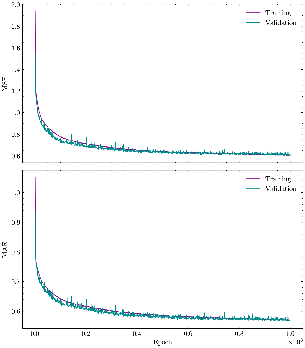
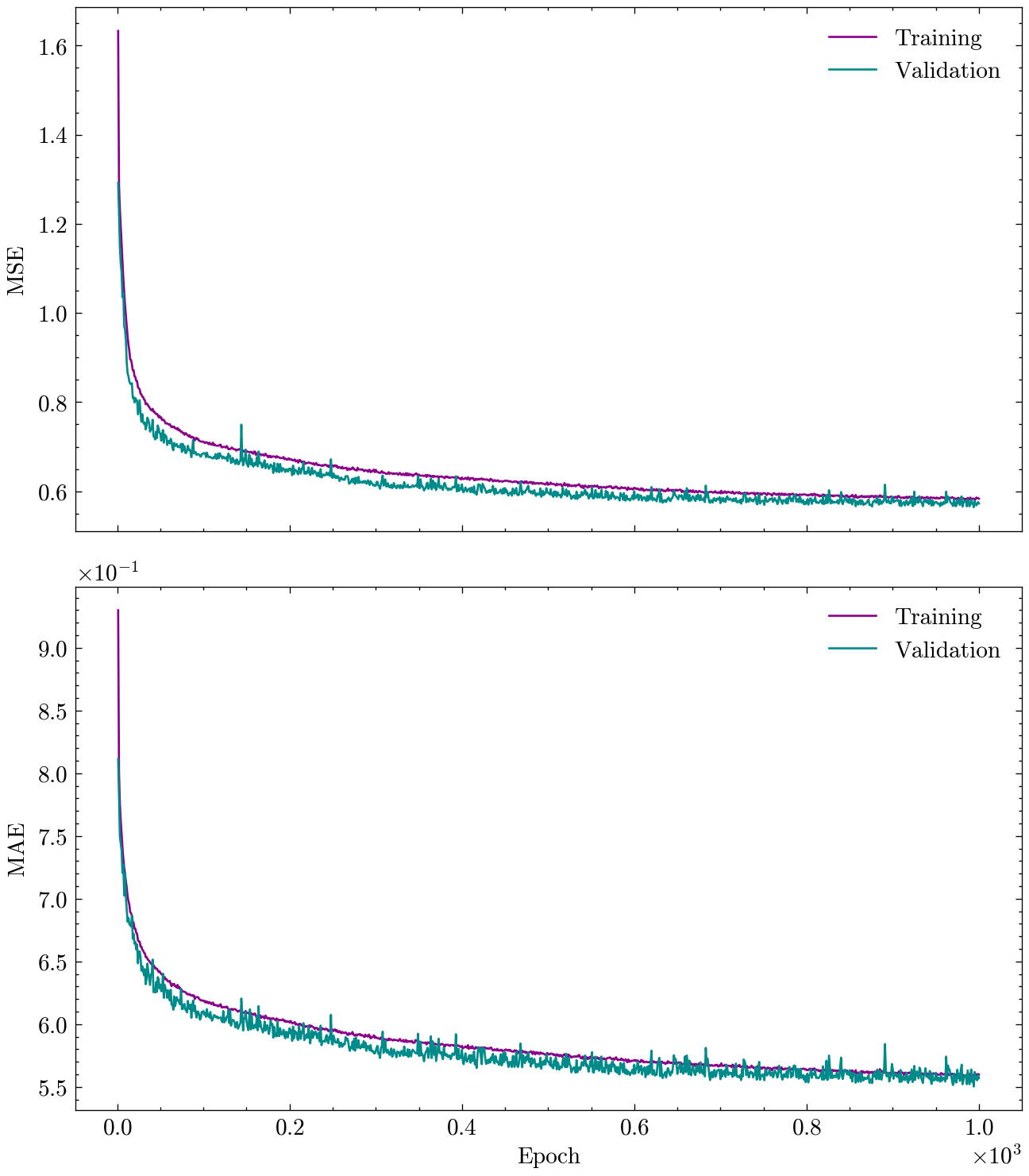
The following figure shows the training and validation loss and metric over epochs.
Code
plot_history(history)
Finally, we can evaluate the trained model on the test set to obtain the final performance metrics.
This value of the MAE is lower than that of the GCN model, confirming the improved performance achieved by the GATv2 model. It is important to note that this improvement has been achieved with a smaller number of parameters (less than 9,000), demonstrating the efficiency and effectiveness of the attention mechanism in capturing relevant information from the graph.
Message Passing Neural Network
To conclude our exploration of GNN architectures, we will implement a Message Passing Neural Network (MPNN). MPNNs represent a highly general and flexible framework for graph neural networks, capable of capturing complex interactions in graph-structured data. The particular MPNN architecture we will implement is based on the GNN layer from (Gilmer et al. 2017). This layer is also known as the edge-conditioned convolution, from (Simonovsky and Komodakis 2017). According to the PyTorch Geometric documentation, the propagation rule for this layer is given by
with \(\vb{F}_e\) a MLP that takes the edge features, \(\vb{e}_{v, u}\), as input and produces a weight matrix of dimensions \(D'\times D\), where \(D\) is the input node feature dimension and \(D'\) is the output node feature dimension. This architecture has been shown to achieve a very good performance on the QM9 dataset, making it a strong candidate for our regression task. However, it is important to take into account that the particular GNN architecture presented here is quite simple and generic to simplify the exposition, and it has not been optimized for this specific task. Therefore, the performance might not match the reported results in (Gilmer et al. 2017) and (Wu et al. 2018).
To build the MPNN model, we will first define a MLP that serves as the edge network, \(\vb{F}_e\). This edge network will consist of two linear layers with a ReLU activation in between. The first layer will project the edge features to a hidden dimension, and the second layer will output a weight matrix that transforms the node features.
Using this edge network, we can now define the MPNN model. The model will consist of two message-passing layers using the NNConv operator from PyTorch Geometric, followed by a global pooling layer and a final MLP to produce the output. A dropout layer will be applied after the first message-passing layer to prevent overfitting.
class MPNN(torch.nn.Module):def__init__(self, num_node_features, num_edge_features, hidden_dim, dropout):super(MPNN, self).__init__()self.dropout = dropout edge_nn1 = EdgeNN(num_edge_features, num_node_features, hidden_dim, hidden_dim)self.conv1 = NNConv(num_node_features, hidden_dim, nn=edge_nn1, aggr='mean') edge_nn2 = EdgeNN(num_edge_features, hidden_dim, hidden_dim, hidden_dim)self.conv2 = NNConv(hidden_dim, hidden_dim, nn=edge_nn2, aggr='mean')self.lin1 = Linear(hidden_dim, hidden_dim)self.lin2 = Linear(hidden_dim, 1)def forward(self, data): x, edge_index, edge_attr = data.x, data.edge_index, data.edge_attr# 1. Obtain node embeddings x = F.relu(self.conv1(x, edge_index, edge_attr)) x = F.dropout(x, p=self.dropout, training=self.training) x = F.relu(self.conv2(x, edge_index, edge_attr))# 2. Readout layer: aggregate node embeddings into a global graph embedding x = global_mean_pool(x, data.batch)# 3. Apply a final regressor x = F.relu(self.lin1(x)) x =self.lin2(x)return x
Again, to keep the model size comparable to the previous models, we will reduce the hidden dimension to 16. The rest of the training setup remains unchanged.
model = MPNN(num_node_features, num_edge_features, 16, 0.05).to(device)optimizer = torch.optim.Adam(model.parameters(), lr=learning_rate)print(f"Number of trainable parameters: {get_total_parameters(model)}")
Number of trainable parameters: 8289
Once again, before training the model, we verify that the model is permutation invariant by permuting the nodes of a molecule and checking that the prediction remains unchanged.
model.eval()print(f'Prediction for the original molecule: {model(molecule).item():.4f}')print(f'Prediction for the permuted molecule: {model(permuted_molecule).item():.4f}')
Prediction for the original molecule: 0.4581
Prediction for the permuted molecule: 0.4581
Now, we can proceed to train the model using the same training loop defined earlier.
history = train(model, optimizer, loss_fn, metric_fn, train_loader, val_loader, epochs)
Epoch 50 ; Training: Loss = 0.7605 Metric = 0.6370 ; Validation: Loss = 0.7072 Metric = 0.6225
Epoch 100 ; Training: Loss = 0.7014 Metric = 0.6121 ; Validation: Loss = 0.6822 Metric = 0.6060
Epoch 150 ; Training: Loss = 0.6765 Metric = 0.6007 ; Validation: Loss = 0.6497 Metric = 0.5911
Epoch 200 ; Training: Loss = 0.6602 Metric = 0.5943 ; Validation: Loss = 0.6317 Metric = 0.5846
Epoch 250 ; Training: Loss = 0.6475 Metric = 0.5878 ; Validation: Loss = 0.6298 Metric = 0.5824
Epoch 300 ; Training: Loss = 0.6368 Metric = 0.5830 ; Validation: Loss = 0.6202 Metric = 0.5796
Epoch 350 ; Training: Loss = 0.6261 Metric = 0.5785 ; Validation: Loss = 0.6202 Metric = 0.5821
Epoch 400 ; Training: Loss = 0.6243 Metric = 0.5780 ; Validation: Loss = 0.6021 Metric = 0.5679
Epoch 450 ; Training: Loss = 0.6199 Metric = 0.5751 ; Validation: Loss = 0.5991 Metric = 0.5669
Epoch 500 ; Training: Loss = 0.6075 Metric = 0.5697 ; Validation: Loss = 0.5954 Metric = 0.5654
Epoch 550 ; Training: Loss = 0.6039 Metric = 0.5678 ; Validation: Loss = 0.6035 Metric = 0.5718
Epoch 600 ; Training: Loss = 0.5988 Metric = 0.5658 ; Validation: Loss = 0.5879 Metric = 0.5584
Epoch 650 ; Training: Loss = 0.5929 Metric = 0.5629 ; Validation: Loss = 0.5784 Metric = 0.5569
Epoch 700 ; Training: Loss = 0.5919 Metric = 0.5622 ; Validation: Loss = 0.5832 Metric = 0.5591
Epoch 750 ; Training: Loss = 0.5898 Metric = 0.5607 ; Validation: Loss = 0.5699 Metric = 0.5536
Epoch 800 ; Training: Loss = 0.5861 Metric = 0.5598 ; Validation: Loss = 0.5830 Metric = 0.5618
Epoch 850 ; Training: Loss = 0.5831 Metric = 0.5573 ; Validation: Loss = 0.5680 Metric = 0.5515
Epoch 900 ; Training: Loss = 0.5840 Metric = 0.5571 ; Validation: Loss = 0.5698 Metric = 0.5549
Epoch 950 ; Training: Loss = 0.5780 Metric = 0.5551 ; Validation: Loss = 0.5669 Metric = 0.5497
Epoch 1000 ; Training: Loss = 0.5724 Metric = 0.5526 ; Validation: Loss = 0.5706 Metric = 0.5536
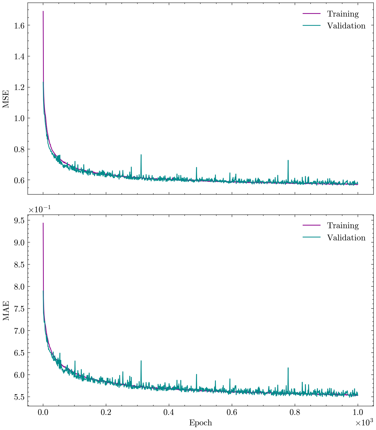
Next, we visualize the training and validation loss and metric over epochs.
Code
plot_history(history)
Finally, we evaluate the trained model on the test set to obtain the final performance metrics.
While this value is similar to that of the GATv2 model, it is far from the ones reported in (Gilmer et al. 2017) and (Wu et al. 2018) (around \(0.3\)). This discrepancy can be attributed to several factors. First, the MPNN architecture implemented here is a simplified version of the one used in those works. Second, the hyperparameters of the model have not been optimized for this specific task. Lastly, this model is the smallest of the three that we have compared. To keep the model size comparable to the previous models, we have reduced the hidden dimension to 16, which might have limited the model’s capacity to learn complex patterns in the data. It is also important to keep in mind that more expressive models do not always guarantee better performance. Simpler models, such as GCNs or GATs, introduce strong inductive biases that can sometimes lead to better results.
Conclusions
Graph Neural Networks open up new possibilities in deep learning, moving from ordered vectors, grids, and sequences to the flexible and relational world of graphs. Graphs are not a niche data type; they are one of the most general and powerful ways to represent complex systems of interactions.
By building the principle of permutation symmetry inherent in graph data directly into their architecture, GNNs provide a powerful and principled framework for learning from a vast range of real-world data. Permutation invariance and equivariance are not just clever architectural tricks; they encode fundamental truths about how relationships in data should be processed. When we force a model to be indifferent to arbitrary node orderings, we eliminate an entire dimension of spurious complexity, allowing the network to focus on learning the actual structural patterns that matter. This represents a profound shift from the brute-force approach of simply throwing more parameters at a problem to one of embedding domain knowledge directly into the architecture. It is the underlying principle of Geometric Deep Learning, a framework that explains the power of many of our most successful models in terms of the symmetries of their data domains they respect. The conclusion is simple: the most successful architectures are not necessarily the most general, but those that encode the right assumptions about the problem structure. This is also the reason why convolutional and attentional GNNs can sometimes outperform more general message-passing networks despite their lower expressiveness: they introduce strong inductive biases that facilitate the learning process.
As we look toward the future, GNNs suggest that the next generation of AI systems will be characterized not by their size, but by their ability to respect and leverage the natural structure of the world. In a sense, GNNs represent a return to first principles: building machines that process information the way the underlying phenomena actually behave. This alignment between computational structure and natural structure may be key to developing AI systems that are not just more powerful, but more interpretable, efficient, and aligned with the systems they aim to model.
Bronstein, Michael M., Joan Bruna, Taco Cohen, and Petar Veličković. 2021. Geometric DeepLearning: Grids, Groups, Graphs, Geodesics, and Gauges. arXiv. https://doi.org/10.48550/arXiv.2104.13478.
Bronstein, Michael M., Joan Bruna, Yann LeCun, Arthur Szlam, and Pierre Vandergheynst. 2017. “Geometric DeepLearning: Going Beyond Euclidean Data.”IEEE Signal Processing Magazine 34 (4): 18–42. https://doi.org/10.1109/MSP.2017.2693418.
Gilmer, Justin, Samuel S. Schoenholz, Patrick F. Riley, Oriol Vinyals, and George E. Dahl. 2017. “Neural MessagePassing for QuantumChemistry.”Proceedings of the 34th InternationalConference on MachineLearning, July, 1263–72. https://proceedings.mlr.press/v70/gilmer17a.html.
Simonovsky, Martin, and Nikos Komodakis. 2017. “Dynamic Edge-ConditionedFilters in ConvolutionalNeuralNetworks on Graphs.”2017 IEEEConference on ComputerVision and PatternRecognition (CVPR) (Honolulu, HI), July, 29–38. https://doi.org/10.1109/CVPR.2017.11.
Veličković, Petar, Guillem Cucurull, Arantxa Casanova, Adriana Romero, Pietro Liò, and Yoshua Bengio. 2018. Graph AttentionNetworks. arXiv. https://doi.org/10.48550/arXiv.1710.10903.
Wu, Zhenqin, Bharath Ramsundar, Evan N. Feinberg, et al. 2018. MoleculeNet: ABenchmark for MolecularMachineLearning. arXiv. https://doi.org/10.48550/arXiv.1703.00564.